
Preparing Time Series Data for LSTM
Stock Price Prediction using Sequence Model


Learning Outcome
5
Reshape 2D data into the required 3D Tensor format
4
Convert a single line of data into "Lookback Windows"
3
Normalize financial data for deep learning stability
2
Split time series data correctly (without leaking the future)
1
Explain why LSTMs cannot directly read a raw column of stock prices
Imagine you are a day trader trying to predict tomorrow's stock price
Bad Startegy
Winning Strategy
You only look at today's closing price: $150.
There is no context, no trend, no pattern.
Result: Predicting tomorrow is almost impossible.
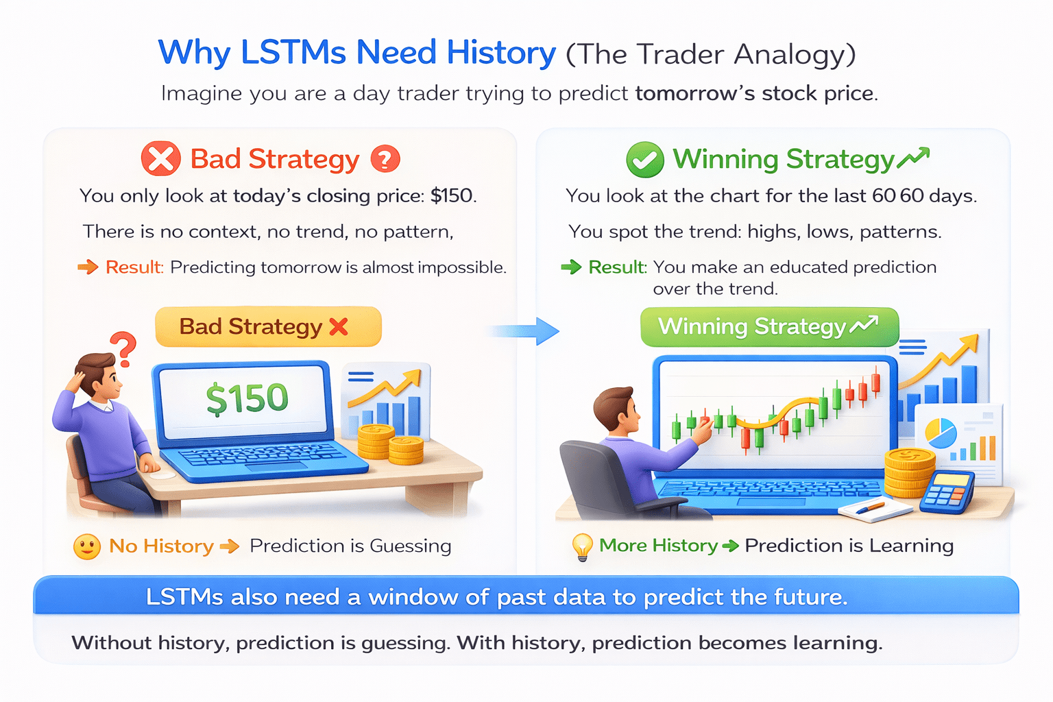
No History
Prediction is Guessing
You look at the chart for the last 60 days.
You spot the trend: highs, lows, patterns
Result: You make an educated prediction over the trend.
More History
Prediction is Learning.
LSTMs act exactly like the winning trader. They need to see a "window" of history.
You only look at today's closing price: $150.
You only look at today's closing price: $150.
You only look at today's closing price: $150.
You only look at today's closing price: $150.
There is no context, no trend, no pattern.
There is no context, no trend, no pattern.
There is no context, no trend, no pattern.
You look at the chart for the last 60 days.
You look at the chart for the last 60 days.
You look at the chart for the last 60 days.
You look at the chart for the last 60 days.
You spot the trend: highs, lows, patterns
You spot the trend: highs, lows, patterns
You spot the trend: highs, lows, patterns
Prediction is Guessing
Prediction is Guessing
Prediction is Guessing
Prediction is Learning.
Prediction is Learning.
Prediction is Learning.
The 4-Step Preparation Pipeline
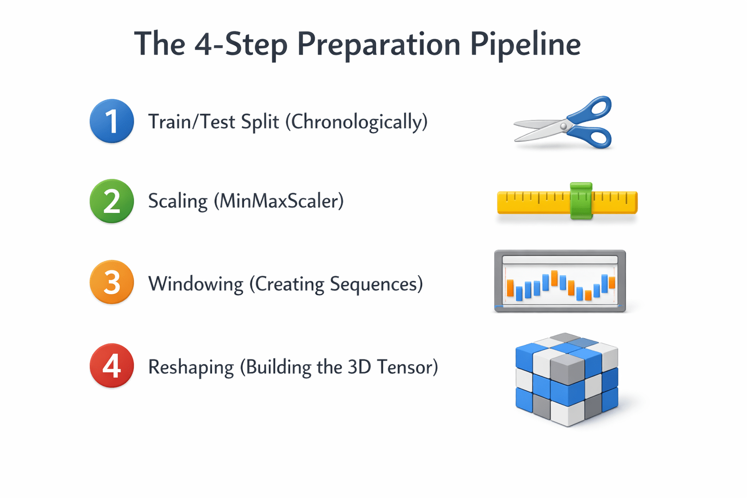
Step 1: The Chronological Split
Warning: Never use train_test_split with random shuffling for time series!

If you randomly shuffle data, you might train the model on Friday's price to predict Wednesday's price. This is "Time Travel" and ruins the model.

Rule: Split by date

Example: Train on 2018-2022 data. Test on 2023 data.
Training
Testing

2018
80%
20%
2023
Rule: Split by date
Example: Train on 2018-2022 data. Test on 2023 data.
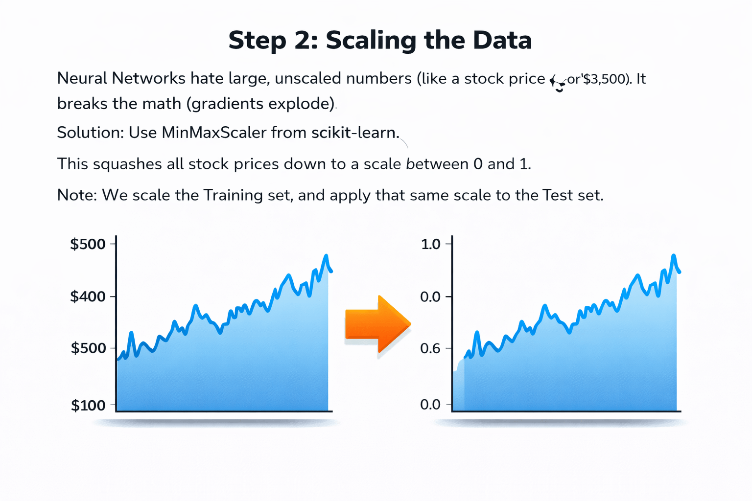
Step 2: Scaling the Data

It breaks the math (gradients explode).
Neural Networks hate large, unscaled numbers
Neural Networks hate large, unscaled numbers
(like a stock price of $3,500).
(like a stock price of $3,500).
It breaks the math (gradients explode).

0.0
0.4
0.6
0.8
1.0
$200
$100
$300
$400
$500

Solution:

Use MinMaxScaler from scikit-learn.
This squashes all stock prices down to a scale between 0 and 1.

Note:
We scale the Training set, and apply that same scale to the Test set.
Use MinMaxScaler from scikit-learn.
This squashes all stock prices down to a scale between 0 and 1.
This squashes all stock prices down to a scale between 0 and 1.
We scale the Training set, and apply that same scale to the Test set.
We scale the Training set, and apply that same scale to the Test set.
We scale the Training set, and apply that same scale to the Test set.
Step 3: Creating Sequences (Windowing)
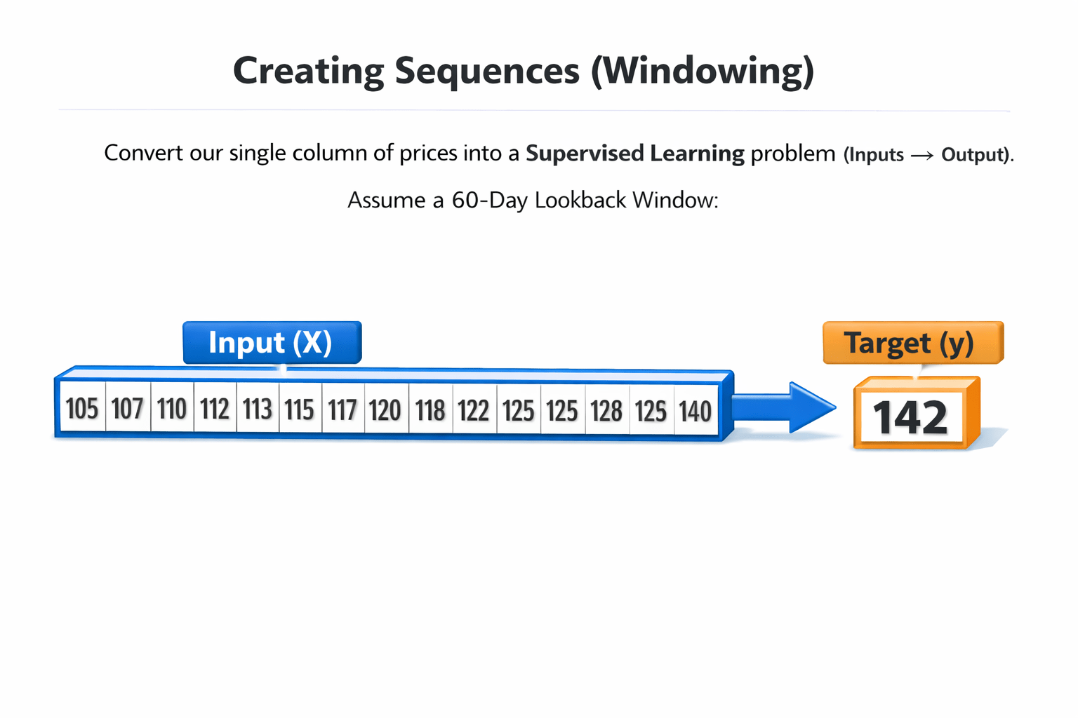
We must convert our single column of prices into a

Supervised Learning problem (Inputs → Output).
Assume a 60-day Lookback Window:

Assume a 60-day Lookback Window:
Assume a 60-day Lookback Window:
Assume a 60-day Lookback Window:
Input (X):
Target (y):
Day 61 price.
Day 1 to Day 60 prices.
Day 1 to Day 60 prices.
Day 61 price.
We must convert our single column of prices into a
Supervised Learning problem (Inputs → Output).
Supervised Learning problem (Inputs → Output).
Supervised Learning problem (Inputs → Output).
We must convert our single column of prices into a
The Sliding Window Concept
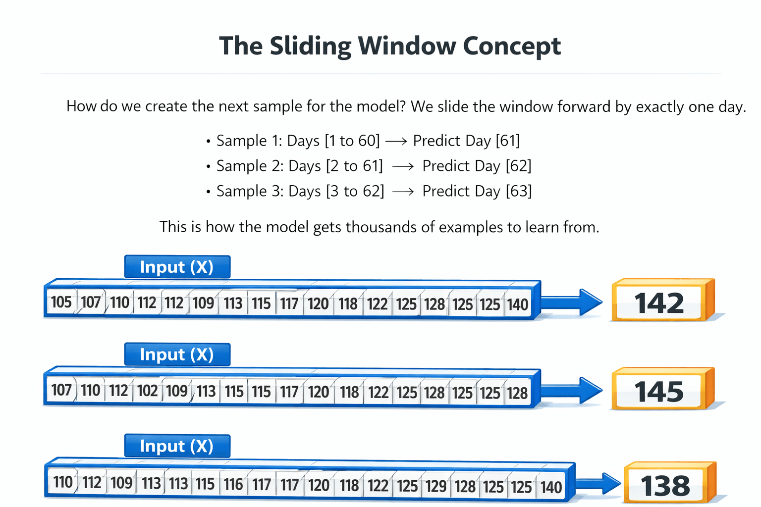
We slide the window forward by exactly one day.
How do we create the next sample for the model?

We slide the window forward by exactly one day.
-
Sample 1: Days [1 to 60] → Predict Day [61]
-
Sample 2: Days [2 to 61] → Predict Day [62]
-
Sample 3: Days [3 to 62] → Predict Day [63]
This is how the model gets thousands of examples to learn from.
This is how the model gets thousands of examples to learn from.
This is how the model gets thousands of examples to learn from.
This is how the model gets thousands of examples to learn from.
This is how the model gets thousands of examples to learn from.
This is how the model gets thousands of examples to learn from.
Step 4: Reshaping for LSTM (The 3D Tensor)
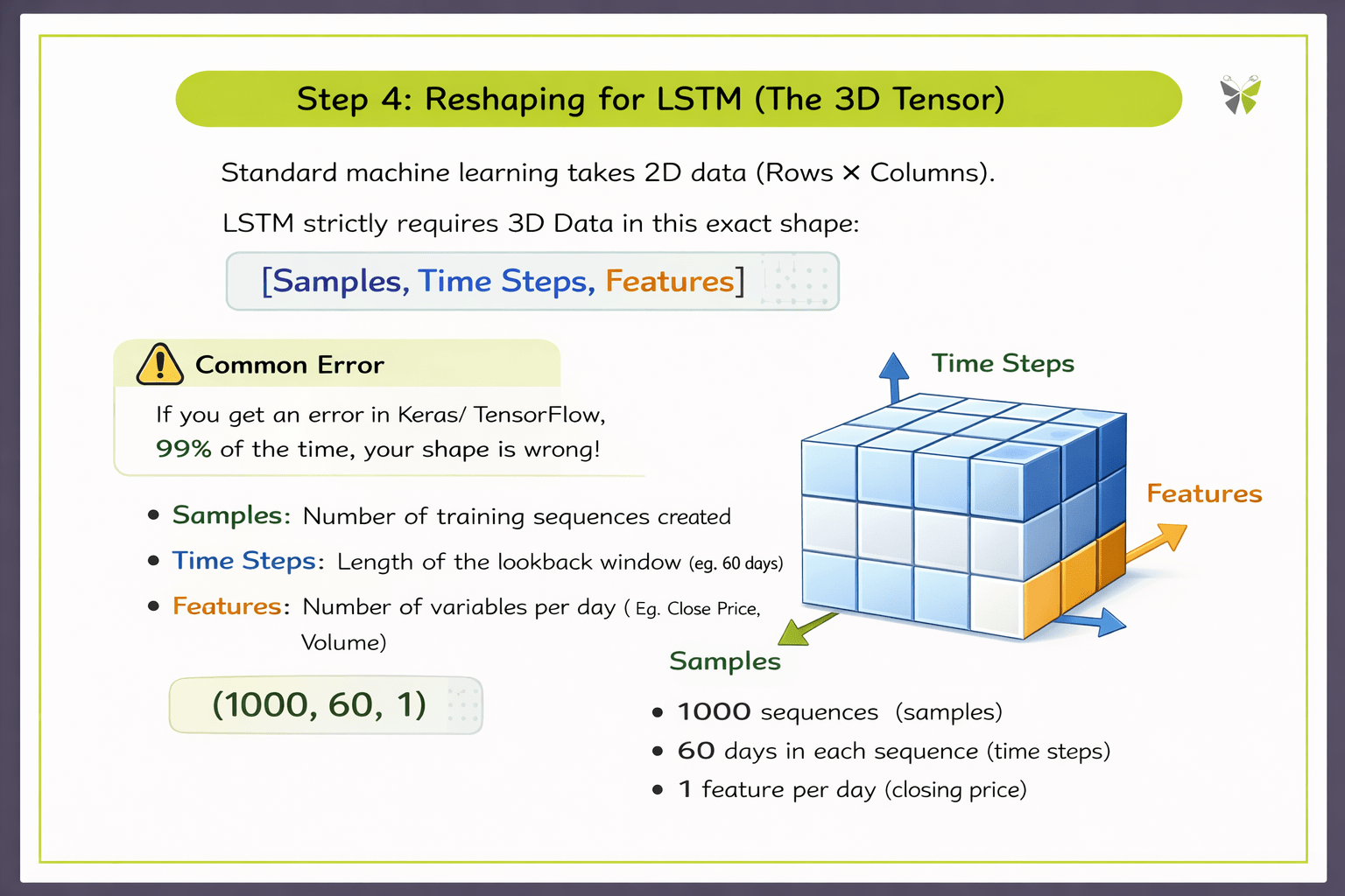
Standard machine learning takes 2D data (Rows & Columns).
LSTM strictly requires 3D Data in this exact format:
[Sample, Time Steps, Features]
Samples: Number of training sequences created
Time Steps: Length of the lookback window
(eg: 60 days)
Features: Number of variables per day (Eg. Close Price, Volume)

If you get an error in Keras/TensorFlow, 99% of the time, your shape is wrong!
Translating the 3D Tensor
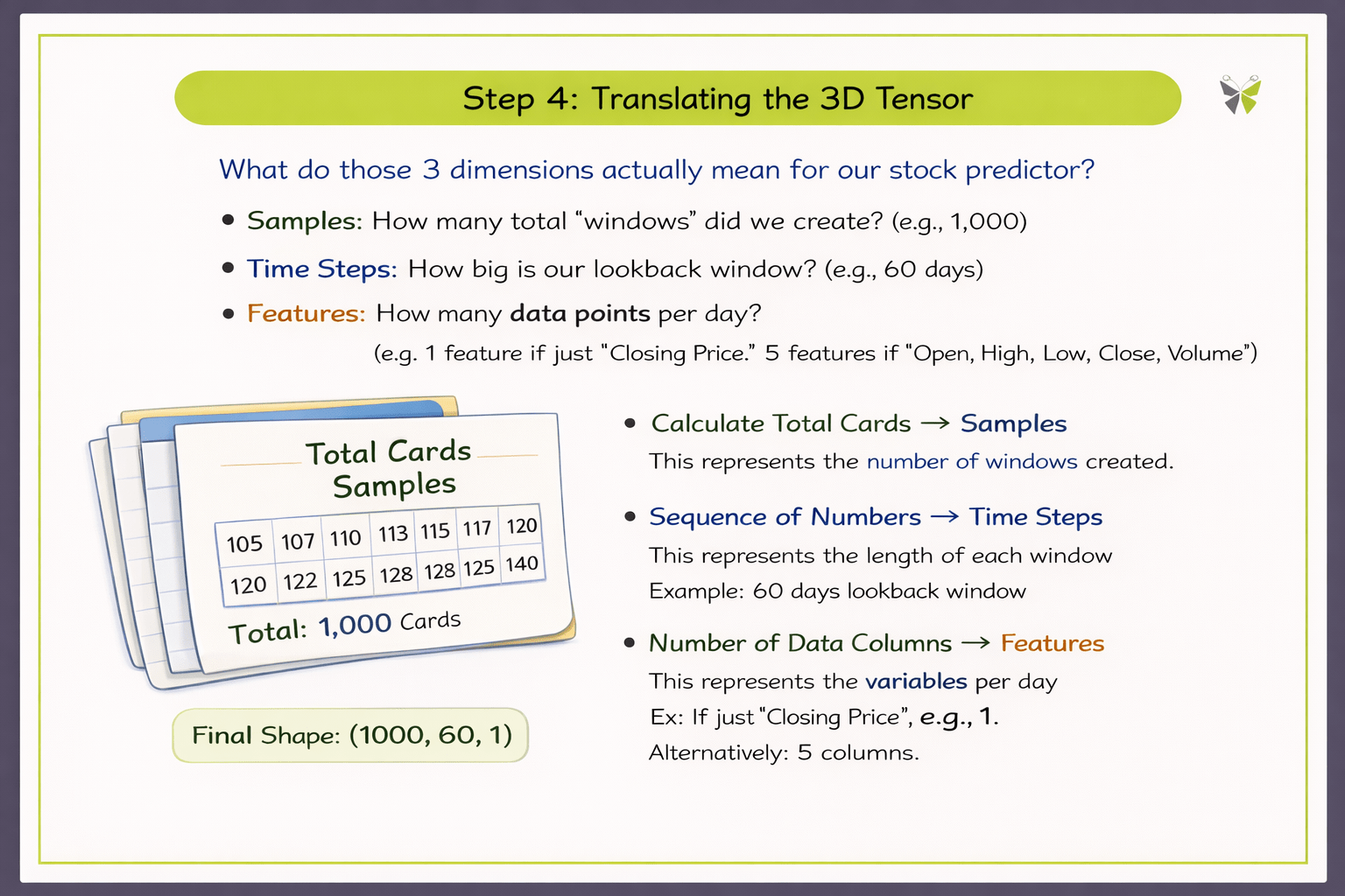
What do those 3 dimensions actually mean for our stock predictor?
Samples:
How many total "windows" did we create? (e.g., 1,000)
Time Steps:
How big is our lookback window? (e.g., 60 days)
Features:
How many data points per day? (e.g., 1 feature if just "Closing Price". 5 features if "Open, High, Low, Close, Volume").
Summary
5
Reshape data to (Samples, Time Steps, Features) for LSTM.
4
Use sliding windows to generate many samples.
3
Create lookback windows (Input → Target).
2
Scale values using MinMaxScaler (0–1 range).
1
Split the data chronologically (no random shuffling).
Quiz
When preparing data for an LSTM model, what does the "Time Steps" dimension represent?
A. The total number of samples in the dataset
B. The length of the lookback window
C. The number of features in the dataset
D. The total number of training epochs

Quiz-Answer

When preparing data for an LSTM model, what does the "Time Steps" dimension represent?
A. The total number of samples in the dataset
B. The length of the lookback window
C. The number of features in the dataset
D. The total number of training epochs