
CVIP 2.0

- Recap of Discriminator models (Neural Networks for function approximation).
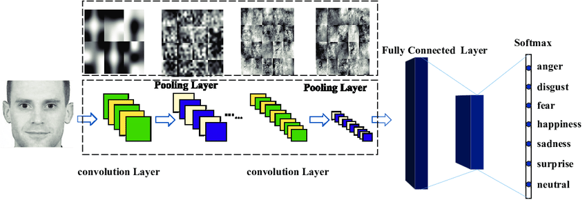
- Deep NNs and CNNs.
- Low-Dimensional features in CNNs.
- Where does data come from?
- What is the structure of a data? What is a distribution?
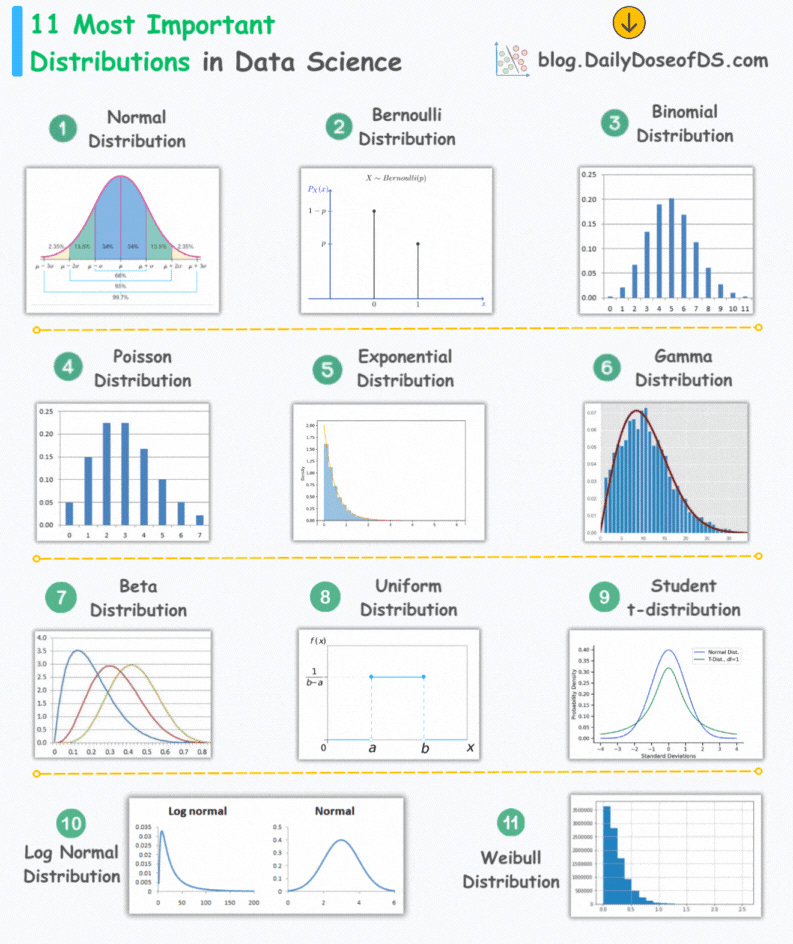
- Types of distributions
- Approximating a distribution
- Why Gaussian Distribution is ubiquitous?
- Bayes rule and Marginalization
- Images as data points
- Interpolation for data generation
\( \text{Agenda of this Lecture:}\)
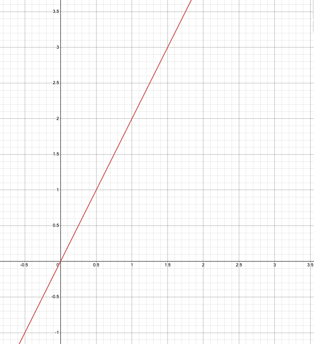
Let's say you are given a bunch of data points:
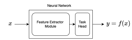
Neural Networks have two components:
- Feature Extractor Module
- Task specific head
You can experiment with simple neural networks at Tensorflow Playground
Usually extracted features are of
lower dimension than data (x)
A simple example of a Neural Network
We have very powerful discriminator models:
- E.g., Image classification models
What about generative models?
Given a label (e.g., "cat"), can we
generate a data point (image)?
Line Fit
Where does the data come from?
Where does the data come from?
Random Experiment
and
Random Variable
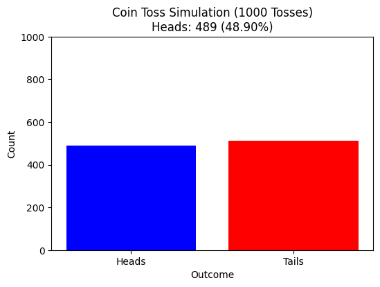
Heads, Tails, Tails, Heads, Heads ......
Guess the random Experiment that gives:
Heads, Tails, Tails, Heads, Heads ......
Guess the random Experiment that gives:
Flipping a coin - of course
Heads
Tails
What can we expect about the outcome?
\( \text{class 0}\)
\( \text{class 1}\)
Decision Boundary
Where does the data come from?
Interpolation for data generation
Can I interpolate between data points?
Basic idea behind morphing images, style mixing, data augmentation
What is the Data Distribution?
What is a Probability Distribution?
A probability distribution describes how the probability mass (discrete) or probability density (continuous) is assigned to different possible outcomes of a random variable.
For a discrete variable X:
For a continuous variable X with PDF \( p(x) \):
What is a Probability Distribution?
- \( p_\theta(x)\) : probability density or mass function parameterized by \( \theta \).
- \( f_\theta(x) \) : energy function or negative log probability
- \( Z_\theta \) : partition function (normalization constant) that ensures the total probability integrates or sums to 1.
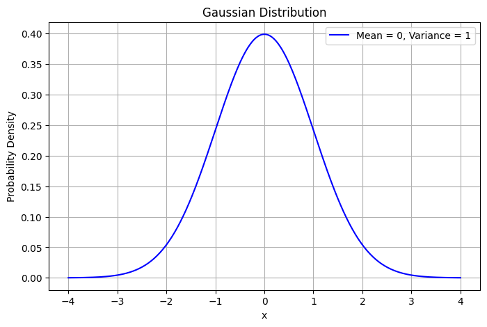
Mean - \( \mu \)
Variance - \( \sigma^2 \)
Variance - \( \sigma^2 \)
change
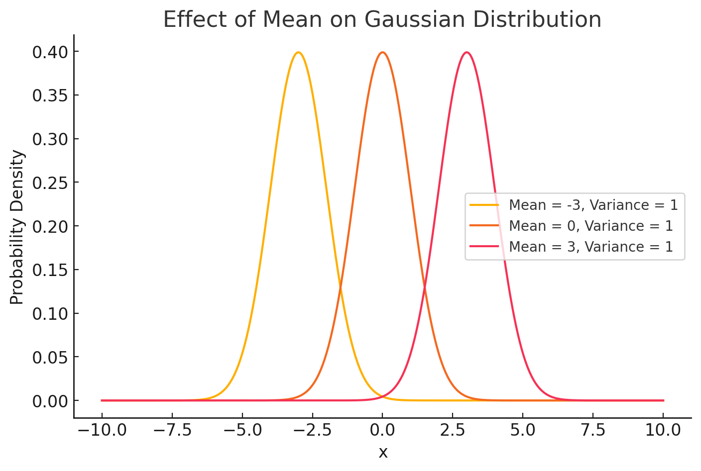
Mean - \( \mu \)
Mean - \( \mu \)
Variance - \( \sigma^2 \)
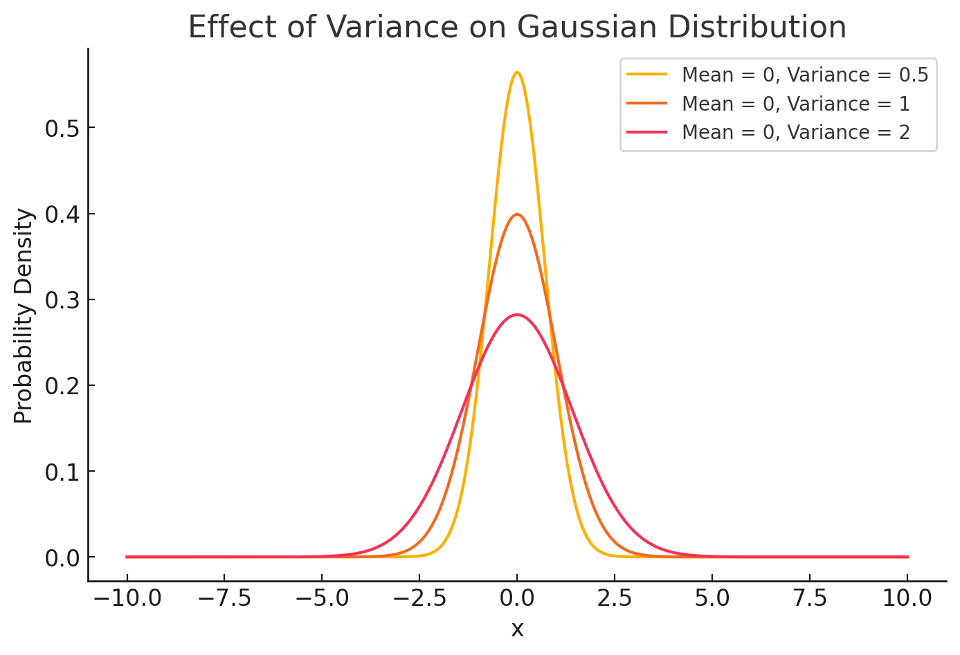
change
Mean - \( \mu \)
Variance - \( \sigma^2 \)
\( x \) follows a normal distribution with mean \( \mu \) and variance \( \sigma^2 \)
Mean - \( \mu \)
Variance - \( \sigma^2 \)
All of these denote Gaussian distributions
A sample from the above distribution:
Suppose \( x_1 \sim \mathcal{N}(\mu_1, \sigma_1^2 I) \) and \( x_2 \sim \mathcal{N}(\mu_2, \sigma_2^2 I) \).
What is the distribution of \( x_1 + x_2 \)?
Suppose \( \boldsymbol{\varepsilon}_1, \boldsymbol{\varepsilon}_2 \sim \mathcal{N}(0, I) \), and
\( \boldsymbol{x}_1 = \sigma_1 \boldsymbol{\varepsilon}_1 \quad \text{and} \quad \boldsymbol{x}_2 = \sigma_2 \boldsymbol{\varepsilon}_2 \)
\( \boldsymbol{x}_1 + \boldsymbol{x}_2 \sim \mathcal{N}(0, (\sigma_1^2 + \sigma_2^2)I) \).
\( \boldsymbol{x}_1 + \boldsymbol{x}_2 = \sqrt{\sigma_1^2 + \sigma_2^2} \, \boldsymbol{\varepsilon} \)
sample
Product of two Gaussians is a Gaussian
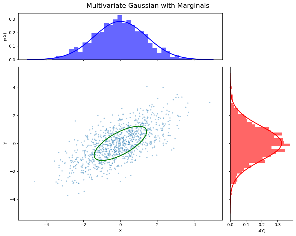
Multivariate Probability Distribution
A multivariate distribution models the joint behavior of multiple random variables simultaneously. For example, a Multivariate Gaussian models the probability of a vector \( \mathbf{x} = [x_1, x_2, …, x_n] \).
General Form:
\( p(\mathbf{x}) = p(x_1, x_2, \ldots, x_n) \)
Joint probability tells us the likelihood of all variables taking specific values together.
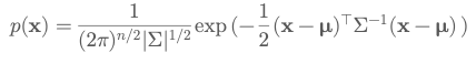
Multivariate Gaussian
Conditional Probability:
Conditional probability quantifies the probability of an event given that another event has occurred.
Reads as: “The probability of x given y”.
Marginalization:
Marginalization is the process of finding the distribution of a subset of variables by summing or integrating out others.
Given \( p(x, y)\), the marginal of \(x\) is:
Interpretation: What is the probability of \( x \), regardless of \(y\)?
Bayes Rule:
Bayes’ Theorem relates conditional probabilities in both directions
Prior
Evidence
Likelihood
Posterior
Expected Value:
The expected value (mean) of a random variable is its long-run average outcome
Represents the “center” of a distribution.
Useful for predictions, variance calculation, and loss expectations.
But, what about images?
Where does your sample come from?


But, what about images?
Where does your sample come from?
unknown
Where does your sample come from?
unknown
But, what about images?
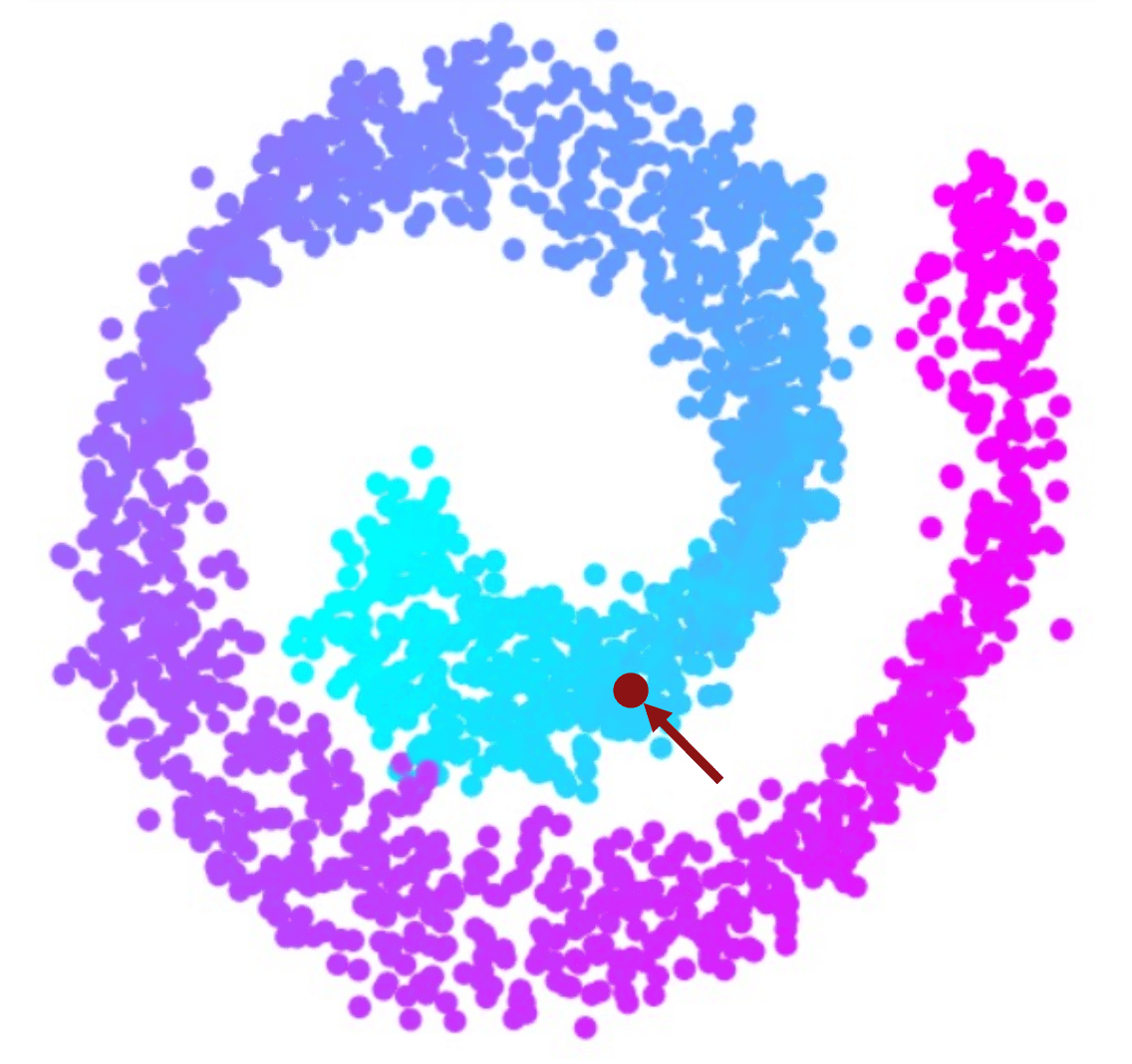
Images are multidimensional vectors
but, what does it mean when two images are closer to each other?
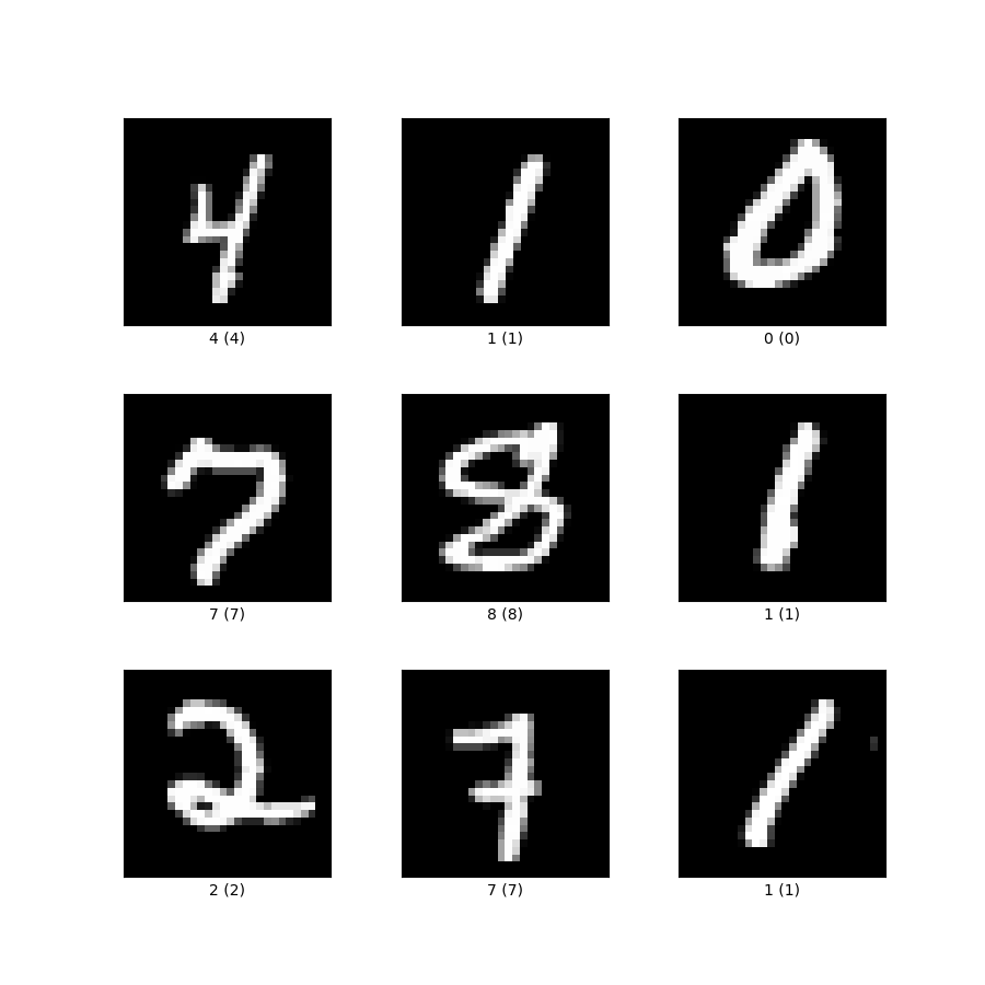
but, what does it mean when two images are closer to each other?
but, what does it mean when two images are closer to each other?
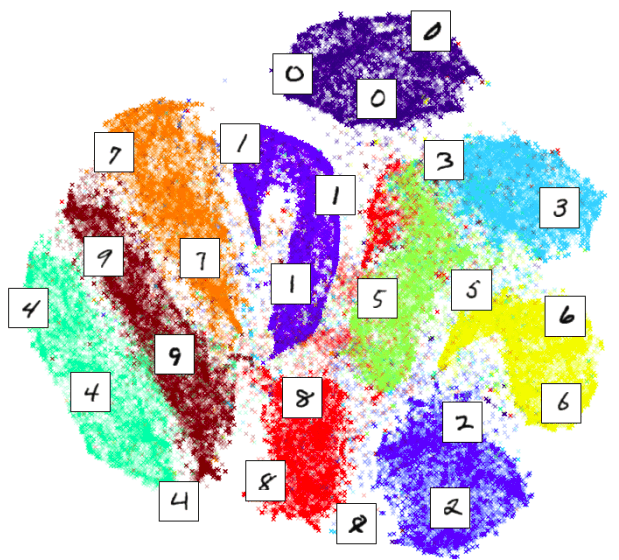
Closer in Low-Dimensional Feature Space