Book 2. Credit Risk
FRM Part 2
CR 9. Estimating Default Probabilities
Presented by: Sudhanshu
Module 1. Credit Ratings and Default Probabilities
Module 2. Credit Default Swaps (CDS)
Module 3. Default Probabilities
Module 1. Credit Ratings and Default Probabilities

Topic 1. Agencies’ Ratings Vs. Internal Credit Rating Systems
Topic 2. Altman's Z-Score
Topic 3. Historical Default Probabilities
Topic 4. Borrowing Rating vs. Probability of Default
Topic 5. Hazard Rates
Topic 6. Recovery Rates
Topic 1. Agencies’ Ratings Vs. Internal Credit Rating Systems
-
Agencies Ratings:
-
Public Availability: Credit rating agencies assign ratings primarily to large, publicly traded bond issuers, and these ratings are available to the general public.
-
Indicator of Credit Quality: Agency ratings signal the overall creditworthiness of an issuer and may change when new positive or negative information becomes available in the market.
-
Long-Term Perspective: Rating agencies focus on long-term creditworthiness, often rating issuers through an economic cycle rather than reacting to short-term fluctuations.
-
Rating Stability: Agencies aim to avoid frequent rating changes, ensuring stability and preventing unnecessary volatility in financial markets.
-
Coverage Limitations: Small and mid-sized firms are often not rated by external rating agencies due to limited public information or lower market relevance.
-
Topic 1. Agencies’ Ratings Vs. Internal Credit Rating Systems
-
Internal Credit Rating Systems:
-
Unrated Borrowers: Financial institutions develop internal rating frameworks to assess the credit risk of unrated borrowers.
-
Key Financial Metrics Used Internally: Internal systems typically evaluate:
-
Profitability: Return on Equity (ROE)
-
Liquidity: Quick Ratio
-
Solvency: Debt-to-Equity Ratio
-
-
Cash Flow Focus: Lenders often adjust company financial statements to derive cash flow statements, which are critical for evaluating a borrower’s ability to repay debt obligations.
-
Topic 2. Altman's Z-score
- Overview: Altman's Z-score is a specific application of Linear Discriminant Analysis (LDA), a statistical method used for creating credit scoring models.
- Purpose: It's used to predict the likelihood of a firm defaulting.
-
Formula: Z=1.2X1+1.4X2+3.3X3+0.6X4+0.999X5
-
Input Variables: The variables (X1 to X5) are a set of five key financial ratios.
- X₁: Working Capital/Total Assets
- X₂: Retained Earnings/Total Assets
- X₃: EBIT/Total Assets
- X₄: Market Value of Equity/Book Value of Total Liabilities
- X₅: Sales/Total Assets
-
Interpreting the Z-Score: The Z-score classifies a firm's credit quality based on a set of guidelines.
-
Z-Score > 3: No default is likely.
-
2.7 - 3: Potential default.
-
1.8 - 2.7: Reasonable probability of default.
-
< 1.8: High likelihood of default.
-
Conclusion: A higher Z-score indicates a higher probability of being solvent, while a lower score suggests a higher risk of insolvency.
-
Practice Questions: Q1
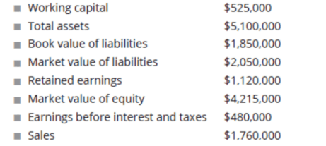
Q1. The following financial data pertains to Nielsen Corp. (Nielsen):
The Altman’s Z-score equation is as follows:
When using the computed Z-score to classify Nielsen based on credit quality, what is the most appropriate classification for the company?
A. No default is likely.
B. Potential default.
C. Reasonable probability of default.
D. High likelihood of default.
Practice Questions: Q1 Answer
Explanation: C is correct.
The five financial ratios for computing Altman’s Z-score are as follows:
1. X1: working capital/total assets = 525,000 / 5,100,000
2. X2: retained earnings/total assets = 1,120,000 / 5,100,000
3. X3: earnings before interest and taxes (EBIT)/total assets = 480,000/5,100,000
4. X4: market value of equity/book value of total liabilities = 4,215,000/1,850,000
5. X5: sales / total assets = 1,760,000 / 5,100,000
Altman’s Z-score is then as follows:
Z = 1.2 × (525,000 / 5,100,000) + 1.4 × (1,120,000 / 5,100,000) + 3.3 × (480,000 / 5,100,000) + 0.6 × (4,215,000 / 1,850,000) + 0.999 × (1,760,000 / 5,100,000)
= 0.1235 + 0.3075 + 0.3106 + 1.3670 + 0.3448 = 2.4534
The following guidelines apply for assessing credit quality:
> 3: no default is likely
2.7-3: potential default
1.8-2.7: reasonable probability of default
< 1.8: high likelihood of default
Therefore, with a Z-score of 2.4534, Nielsen has a reasonable probability of default.
Topic 3. Historical Default Probabilities
-
S&P borrowing ratings: Ratings range from AAA (highest rating; best quality) to D (lowest rating; in payment default).
-
Investment-grade bonds are rated AAA to BBB, while non-investment-grade ("junk") bonds are BB to D.
-
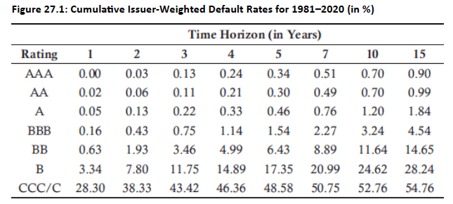
- Cumulative probabilities of default: A bond with an AA rating has a 0.02% chance of defaulting by the end of Year 1 and a 0.06% chance by the end of Year 2.
- Marginal Probability of Default: The probability that a default will occur within a specific year, given that it hasn't defaulted before that year.
-
Example (AA-rated bond): The marginal probability of defaulting in Year 3 is the cumulative probability at the end of Year 3 minus the cumulative probability at the end of Year 2 = 0.11%−0.06%=0.05%.
Practice Questions: Q2
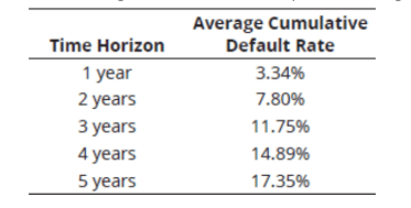
Q2. The following information is an excerpt from a rating migration matrix for a B-rated bond:
What is the probability that the bond will default during the fourth year conditional on no earlier default?
A. 2.46%.
B. 2.79%.
C. 3.14%.
D. 3.56%.
Practice Questions: Q2 Answer
Explanation: D is correct.
The probability of a B-rated bond defaulting in the fourth year is 14.89% - 11.75%= 3.14%.
The probability that the bond will survive until the end of the third year is 100%- 11.75% = 88.25%.
Thus, the probability that the bond will default during the fourth year conditional on no earlier default is computed as 3.14% / 88.25% = 3.56%.
Topic 4. Borrowing Rating vs. Probability of Default
- The Relationship: In general, a lower borrowing rating generally corresponds to a higher probability of default, and a higher rating corresponds to a lower probability of default.
-
Marginal PD Behaviour Over Time:
-
For investment-grade bonds and some non-investment-grade bonds, the marginal probability of default (PD) typically increases over time during the initial years.
- This reflects the assumption that an issuer may appear financially stable at the outset, but as time progresses, uncertainty and the potential for financial deterioration gradually increase, leading to a higher likelihood of default in later periods.
-
For certain non-investment-grade bonds, the marginal probability of default may decline over time because the initial years are the most critical for survival.
- If the issuer avoids default during early periods, it suggests that the firm’s financial condition may be more stable than initially perceived, leading to lower incremental default probabilities in later years.
-
For investment-grade bonds and some non-investment-grade bonds, the marginal probability of default (PD) typically increases over time during the initial years.
Topic 5. Hazard Rates
- Hazard Rate: The hazard rate is also called the conditional default probability. It is the probability of default within a specific period, conditional on no earlier default.
-
Calculation: Conditional default probability = (Unconditional default probability) / (Probability of no earlier default).
-
Example: For a BB-rated bond in Year 4, the unconditional default probability is 1.53%. The probability of no earlier default (by the end of Year 3) is 100% - 3.46% = 96.54%.
-
The conditional default probability (hazard rate) is 1.53%/96.54%=1.58%.
-
Formula: The probability of default by time t can be approximated with the average hazard rate (λ(t)):
-
-
-
-
From Fig 27.1, the unconditional default probability for BB-rated bond in Year 4 (from a Year 0 perspective) is 1.53% (= 4.99% - 3.46%).
-
The probability that the BB-rated bond remains in place until the end of Year 3 is 96.54% (= 100% - 3.46%).
-
Conditional default probability: Probability that the bond will default in Year T, conditional on no earlier default. The conditional default probability that the bond will default in Year 4 is: 1.58% (= 1.53% / 96.54%).
-
Hazard rate: If one year is considered a sufficiently short amount of time, then the conditional default probability could also be called the hazard rate of default intensity.
-
Formula for probability of default by time t:
-
-
-
Assuming a constant hazard rate of 2% per year,
-
The probability of default by the end of Year 1 (t = 1)
-
The probability of default by the end of Year 2 (t = 1)
-
-
Therefore, the unconditional probability of default during Year 2 = 3.92%-1.98%=2.94%
-
Also, the conditional probability of default in Year 5, conditional on no earlier default, is:
-
2.94%/(1-1.98%)=2.99%
-
Topic 5. Hazard Rates
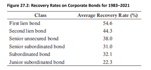
Topic 6. Recovery Rates
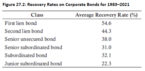
- Definition: A recovery rate is the percentage of the face value of a debt that creditors are likely to recover in the event of a default or bankruptcy.
- Seniority: More senior bonds have higher average recovery rates than more junior bonds.
-
Recovery rates on debt are typically negatively correlated with default rates. For example, in mortgage markets, higher default rates lead to more foreclosures and increased housing supply, which pushes property prices downward and ultimately reduces the lender’s recovery value on the collateral.
-
In a strong economic environment, bond default rates are generally low, and when defaults occur, recovery rates tend to be higher due to better asset values and stronger market conditions.
Topic 6. Recovery Rates
-
In contrast, during a weak economic environment, bond defaults increase, and the average recovery rate declines because distressed assets lose value and liquidity becomes limited.
-
This creates a negative correlation between default rates and recovery rates, which is particularly challenging for lenders in downturns since they face both higher default frequency and lower recoveries simultaneously.
-
Example (Mortgages): Higher mortgage default rates lead to more foreclosures and a surplus of properties on the market, which in turn drives down property prices and reduces the lender's recovery rate.
Topic 6. Recovery Rates
Module 2. Credit Default Swaps (CDS)
Topic 1. CDS and its Mechanics
Topic 2. Credit Indices
Topic 3. Fixed Coupons
Topic 4. CDS Spreads
Topic 5. CDS-Bond Basis
Topic 6. Approximating Hazard Rates
Topic 7. Most Precise Hazard Rates
Topic 1. CDS and its Mechanics
-
CDS: A credit derivative where one party makes payments to another for credit protection.
- The CDS purchaser seeks credit protection (default protection buyer) makes regular, usually quarterly, payments to the seller (default protection seller).
- The seller agrees to pay the buyer a pre-specified amount if a credit event occurs.
- Credit events can include non-timely payment, debt restructuring, or bankruptcy.
- Underlying Entity: The CDS is based on a specific company, or "reference entity".
-
Settlement: If a credit event occurs, the swap can be settled in two ways:
- Physical Delivery: The seller pays the buyer the notional principal of the bonds and receives the defaulted bonds in exchange. The contract often specifies a list of acceptable bonds that can be delivered.
-
Cash Settlement: Dealers are surveyed to determine the mid-point between bid and ask prices of the cheapest-to-deliver (CTD) bond. The cash payoff is then the difference between the face value and the market value of the bond.

Topic 1. CDS and its Mechanics
-
Example: Suppose FI Advisors (FIA) owns fixed-income securities issued by ELF Corp. (ELF, the reference entity) with a par value of $200 million.
- FIA would like to protect its position against credit risk by using a CDS and is able to purchase such protection from Market Makers, Inc. (MM) for 75 basis points (i.e., the CDS spread) of a notional principal of $200million on September 20, 2024.
- The life of the CDS is 5 years, which will require FIA to pay the equivalent of $1.5 million (= $200 million X 0.0075) to MM every year (or about $375,000 per quarter on the standard maturity dates of Mar 20, Jun 20, Sep 20 and Dec 20).
- No default: If ELF does not default, then FIA receives nothing from the swap.
-
Default:
-
Physical Settlement: If ELF defaults (e.g., Jul 20, 2028), MM pays $200 million (notional) to FIA and receives the ELF bonds, which must come from a predefined list of eligible deliverable bonds.
-
Cash Settlement: the payoff is based on the cheapest-to-deliver (CTD) bond price determined by dealer quotes; if the CTD bond trades at $0.40 per dollar of face value, FIA receives 60% of notional ($120 million).
-
- The protection buyer pays the premium to the protection seller only until there is a credit event. In above example, a final accrual payment of about $125,000 (= $375,000 per quarter X 1/3) to cover the one-month period from June 20, 2028 to July 20, 2028 is required.
Topic 1. CDS and its Mechanics
- Maturities of CDS Contracts: CDS contracts are traded with maturities that include 1, 2, 3, 5, 7, and 10 years, with 5 years being the most common in practice.
- Due to the standard maturity dates, the actual life of the CDS contract might not be identical to the stated life, but it will be close.
-
For example, a CDS that is initiated on Aug 10, 2025 would probably mature on Sep 20, 2030.
- The fiirst payment due on Sep 20, 2025 would be an accrual amount to account for the period from August 10 to September 20, 2025.
- Subsequently (e.g., Dec 20, 2025 payments and onward), the quarterly payments would be fixed.
Topic 2. Credit Indices
- Credit indices are portfolios of CDSs that allow investors to trade credit risk on a broad basket of reference entities.
-
Two well-known investment-grade credit indices, both of which have 125 reference entities and maturities commonly of 3, 5, 7, and 10 years are
- CDX NA IG (North America) and
- iTraxx Europe.
-
Example: An investor buying protection on the 5-year iTraxx Europe index at an ask price of 152 bps for €500,000 per firm would make total annual payments of 0.0152×€500,000×125=€950,000.
- If one reference entity defaults, the investor receives the appropriate payoff and a future reduction in annual payments of €7,600 (€950,000/125).
Practice Questions: Q1
Q1. The five-year CDX NA IG Index (125 companies) is quoted as bid 141 bps and ask 143 bps. An investor plans to sell $1 million of protection on each company. At the beginning of the third year before the annual protecon payment, one of the companies defaults. Assuming no other defaults, the investor’s cash flow for the third year is closest to:
A. $748,400 inflow.
B. $748,400 outflow.
C. $773,200 inflow.
D. $773,200 outflow.
Practice Questions: Q1 Answer
Explanation: A is correct.
The investor will sell CDS protection on the 125 companies in the index for 140 bps per company. The annual receipt by the seller is 0.0141 × $1,000,000 × 125 = $1,762,500. However, because one company defaulted before the protection payment, the annual receipt by the CDS seller will be reduced by $1,762,500 / 125 = $14,100. In addition, the seller will have to pay $1 million to the CDS protection
buyer as a result of the default. The CDS seller’s cash inflow for the year is computed as $1,762,500 - $14,100 - $1,000,000 = $748,400.
Topic 3. Fixed Coupons
- In a CDS contract, the protection buyer pays a regular fixed coupon to the protection seller in return for default protection.
- For investment-grade issuers, this fixed coupon is standardized to 100 basis points (1%) to simplify contract settlement and clearing.
- This standardized coupon is not necessarily the fair premium or CDS spread.
- An up-front premium may be paid to bridge the gap between the standardized fixed coupon and the fair CDS spread.
-
There are three possibilities for the up-front premium:
-
CDS spread = fixed coupon: No up-front premium is paid.
-
CDS spread > fixed coupon: The protection buyer pays an up-front premium equal to the present value of (CDS spread - fixed coupon).
-
CDS spread < fixed coupon: The protection seller pays an up-front premium to the protection buyer, equal to the present value of (fixed coupon - CDS spread).
-
Topic 4. CDS Spreads
- CDS spread is the price of the CDS, expressed in basis points. It represents the annual premium that the protection buyer pays to the protection seller for bearing the credit risk.
- Bond Yield Spread: Excess of the corporate bond yield over a comparable risk-free bond. In theory, the CDS spread should equal the bond yield spread
-
Arbitrage: If the CDS spread and bond yield spread are not equal, an arbitrage opportunity may exist:
-
CDS spread < bond yield spread: Buy the corporate bond and buy CDS protection to earn more than the risk-free rate.
-
CDS spread > bond yield spread: Sell the corporate bond and sell CDS protection to borrow at less than the risk-free rate.
-
-
Example: A 5-year corporate bond yielding 6% can be hedged by purchasing a 5-year CDS with a spread of 1.5%, transferring the credit risk to the CDS seller.
-
After paying the CDS premium, the net return becomes 4.5% (6% − 1.5%), which effectively represents the implied risk-free return if the bond does not default.
-
If a default occurs, the investor earns 4.5% until default, and the CDS payoff compensates the loss by returning the bond’s face value, which can then be reinvested at the risk-free rate for the remaining period.
-
Practice Questions: Q2
Q2. In the context of arbitrage trades, if the CDS spread is significantly greater than the bond yield spread, what is the most appropriate action by the investor?
A. Buy the corporate bond and buy CDS protection.
B. Buy the corporate bond and sell CDS protection.
C. Sell the corporate bond and buy CDS protection.
D. Sell the corporate bond and sell CDS protection.
Practice Questions: Q2 Answer
Explanation: D is correct.
If the CDS spread is greater than the bond yield spread, sell the corporate bond, and sell CDS protection to borrow at less than the risk-free rate.
Topic 5. CDS-Bond Basis
-
The CDS-bond basis is defined as the difference between the CDS spread and the bond yield spread.
- CDS-bond basis = CDS Spread - bond yield spread
-
Although CDS-bond basis should be theoretically zero, it is often non-zero in practice due to several factors.
-
Bonds trading significantly above or below par
-
Counterparty risk in CDS contracts (negative basis)
-
The possibility of a CTD bond in a CDS (positive basis)
-
CDS payoffs excluding accrued interest (negative basis)
-
Restructuring clauses in CDS contracts allowing for payoffs, even without default (positive basis)
-
The bond yield spread is computed using a risk-free rate that is dissimilar to the one used by the market
-
Illiquidity, which prevents full exploitation of arbitrage opportunities.
-
- The basis was generally positive before the 2007-2009 financial crisis but has since become negative and less significant.
Topic 6. Approximating Hazard Rates
-
An approximate calculation for the average hazard rate can be derived from credit spreads for a bond trading near par value.
-
-
-
s(T) is the credit spread for maturity T and RR is the recovery rate.
-
-
-
Example: With a 5-year credit spread of 210 bps (2.1%) and a recovery rate of 30%, the average annual hazard rate is 0.021/(1−0.3)=3%.
-
Bootstrapping a Term Structure: This method can be used to determine a term structure of hazard rates from credit spreads for different maturities.
-
For a 3-year spread of 80 bps and a 65% recovery rate, the average 3-year hazard rate is 0.008/(1−0.65)=2.29%.
-
For a 5-year spread of 90 bps and 65% recovery, the average 5-year hazard rate is 0.009/(1−0.65)=2.57%.
-
The average hazard rate between Year 3 and Year 5 is then [(5×0.0257)−(3×0.0229)]/2=2.99%.
-
The average hazard rate between Year 5 and Year 10 is: [(10×0.0314)−(5×0.0257)]/2=3.71%.
-
Topic 7. More Precise Hazard Rates
-
For bonds that do not trade near their par value, a more precise calculation is required which involves comparing the price of a risky corporate bond to a comparable risk-free government bond.
- The difference in their prices represents the expected loss from default over the bond's term.
- The present value of the expected loss is calculated based on assumed default probabilities at specific times, usually before coupon payment dates.
- The default probability (
-
Consider a 5-year risky corporate bond with a 6% annual coupon (paid semiannually) and a 7% continuously compounded yield, resulting in a price of 95.34 for a face value of 100.
-
A comparable risk-free government bond with the same coupon structure but a 5% continuously compounded yield is priced higher at 104.09.
-
The difference in prices arises because the risky bond incorporates credit risk and the possibility of default, while the government bond is assumed to be default-free.
-
The price gap of 8.75 (104.09 − 95.34) represents the market’s estimate of the expected loss due to default over the 5-year life of the corporate bond.
-
Topic 7. More Precise Hazard Rates
-
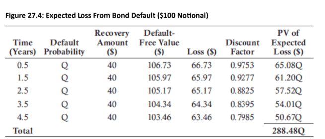
Fig 27.4 shows the computation of the PV of expected loss assuming that bond defaults can occur only at five specified points in time, each immediately before scheduled coupon payment dates. A constant default probability QQQ is assumed throughout the bond’s life, with a fixed RR of 40% applied to the bond value in the event of default.
-
The expected value of a default-free bond at t = 4.5 years is 103.46, calculated as:
-
-
-
With RR as 40% of the face value, LGD is 63.46 (= 103.46 - 40), and on a discounted basis using a 5% annual discount rate, the loss is 50.67 and the expected loss is 50.67Q.
-
From Fig 27.4, the total expected loss for all the periods is 288.48Q. Given the 8.75 amount computed earlier, the default probability (Q) = 8.75/288.48 = 3.03%.
Topic 7. More Precise Hazard Rates
-
Using a sample of bonds maturing in 2, 5, and 7 years, a bootstrapping process could be used for estimating the term structure of default probabilities.
-
the 2-year bond could be used to estimate the default probability for the first two years,
-
the 5-year bond to estimate the annual default probabilities for Years 4 and 5,
-
the 7-year bond to estimate the annual default probabilities for Years 6 and 7.
-
Module 3. Default Probabilities
Topic 1. Default Probabilities Estimation
Topic 2. Real-World vs. Risk-Neutral Default Probabilities
Topic 3. Default Probability Using Merton Model
Topic 4. Merton Model Performance
Topic 1. Default Probabilities Estimation
-
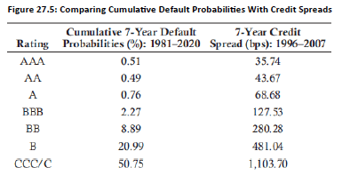
Fig 27.5 provides the 7-year average cumulative default probabilities for issuers of varying credit ratings (from S&P in Column 1) and the 7-year credit spread for varying ratings (from Merrill Lynch in Column 2).
-
The values in Figure 27.5 can be used to estimate the average 7-year hazard rates using two calculation methods.
-
The first method applies the following equations:
-
-
Method 1: A BBB-rated issuer has a cumulative 7-year default rate of 2.27%, so the average hazard rate is calculated as:
-
-
Method 2: Using the same BBB-rated issuer as Method 1, but using the 7-year credit spread and a 40% recovery rate assumption, the average 7-year hazard rate is:
-
-
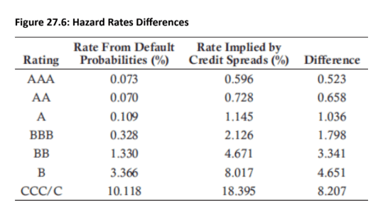
A summary of the average 7-year hazard rates is provided in Fig 27.6 for the full range of credit ratings using the same methodologies just discussed.
Topic 1. Default Probabilities Estimation
-
From Fig 27.6, hazard rates implied from credit spreads are significantly higher than those estimated from historical default data.
-
The gap between the two hazard rates is smaller for higher credit quality and larger for lower credit quality instruments, suggesting that credit spreads compensate investors more than the expected default losses.
-
The excess compensation becomes more pronounced for lower-rated instruments and during periods of economic stress with high spreads.
-
Bond defaults are influenced by economic conditions rather than being independent; strong economies tend to reduce default probabilities, while weak economies increase them.
-
Historical data shows large year-to-year variation in default rates, creating systematic (non-diversifiable) risk that cannot be eliminated through diversification.
-
Because lower-quality debt behaves similarly to equity in terms of risk, investors demand higher expected and excess returns as compensation for the additional risk.
Topic 1. Default Probabilities Estimation
-
Unlike equities, it is often difficult or impractical to fully diversify away unsystematic risk in a bond portfolio.
-
Investors may deliberately take on unsystematic credit risk because it can offer additional return through higher credit spreads.
-
Corporate bonds are generally less liquid than government bonds, so part of the higher credit spread compensates investors for liquidity risk.
Topic 2. Real-World vs. Risk-Neutral Default Probabilities
-
Risk-neutral assumption: Expected asset growth equals the risk-free rate
-
Real-world assumption: Expected asset growth = risk-free rate + market risk premium
-
Impact on asset valuation: Higher expected growth in the real world leads to higher asset values
-
Effect on default probability: For the same debt face value, real-world default probability < risk-neutral default probability
-
Use-case distinction
-
Risk-neutral estimates suit valuation (e.g., credit spreads)
-
Real-world estimates suit scenario analysis (e.g., historical default data)
-
Topic 3. Default Probability Using Merton Model
-
Merton Model: The Merton model treats a company's equity as a call option on the company's assets.
-
For this model, we assume that there is debt outstanding that needs to be repaid at time T.
-
Key Variables: The model uses the following variables to compute default probability:
-
V0V_0V0: Current value of the firm’s assets
-
VTV_TVT: Value of the firm’s assets at time TTT
-
D: Total debt due at time TTT
-
E0: Current value of the firm’s equity
-
ETE_TET: Equity value at time TTT, defined as max(VT−D,0)\max(V_T - D, 0)max(VT−D, 0)
-
σV\sigma_VσV: Volatility of firm asset value
-
σE\sigma_EσE: Volatility of equity value
-
-
The strike price of the call option is the total debt to be repaid (D). Therefore,
-
ET=max(VT−D,0)E_T = \max(V_T - D, 0)ET=max(VT−D,0)
-
-
The above solvency condition makes sense because
-
If VT>DV_T > DVT>D: firm services debt and equity retains positive value
-
If VT<DV_T < DVT<D: default is optimal since equity value becomes zero
-
-
-
With no dividends assumption, the Black-Scholes-Merton equity value today is:
-
-
-
-
-
Using calculus, we can derive below equation:
-
- Once V0V_0V0 and σV\sigma_VσV are determined, d1d_1d1, d2d_2d2, N(d1)N(d_1)N(d1), and N(−d2)N(-d_2)N(−d2) can be computed directly.
- Risk-neutral probability of default: When the option is not exercised, there is a default by the firm, the risk-neutral probability of firm default is denoted as
-
Distance to Default (DD): The number of standard deviations that the asset price must fall to lead to a default at time T. The higher (lower) the distance to default, the lower (higher) the probability of default. It can be calculated as:
-
Topic 3. Default Probability Using Merton Model
Practice Questions: Q1
Q1. A junior analyst is evaluating the following questions to include in her research report:
- Which type of default probabilities should be used in valuation?
- What is the impact on a company defaulting when the distance to default rises?
Regarding these questions, the analyst’s report should support which of the following conclusions?
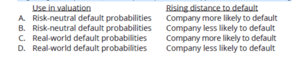
Practice Questions: Q1 Answer
Explanation: B is correct.
Risk-neutral default probabilities should be used in valuation, and real-world default probabilities should be used in scenario analysis. As the distance to default rises (falls), the company is less (more) likely to default.
Topic 4. Merton Model Performance
-
Empirical studies show that the Merton, Moody’s-KMV, and Kamakura models produce reliable and accurate rankings of default probabilities.
-
The Merton model estimates risk-neutral default probabilities, derived from option pricing theory.
-
Moody’s-KMV and Kamakura transform Merton’s output into real-world (physical) default probabilities.