Binary Black Holes
A GENERIC Approach
Ref Bari
Advisor: Prof. Brendan Keith


The Goal
The Goal
Can a Neural Network learn ?
The Goal
Can a Neural Network learn ?
Starting from ?
The Goal
Can a Neural Network learn ?
Starting from ?
Starting from ?
Training on
The Goal
Can a Neural Network learn ?
Starting from ?
Starting from ?
Training on
In the GENERIC Formalism?
The Goal
Can a Neural Network learn ?
Starting from ?
Starting from ?
Training on
In the GENERIC Formalism?
Learnable Parameters:
Correction to Hamiltonian
The Answer
It seems like it!*
*Major caveats lie ahead
The Recipe
- Generate Training Data
- Define Hamiltonian in GENERIC Form
- Define Neural ODE
- Create Loss + Callback Functions
- Optimize over Learnable Parameters
- Iteratively Train the Optimizer
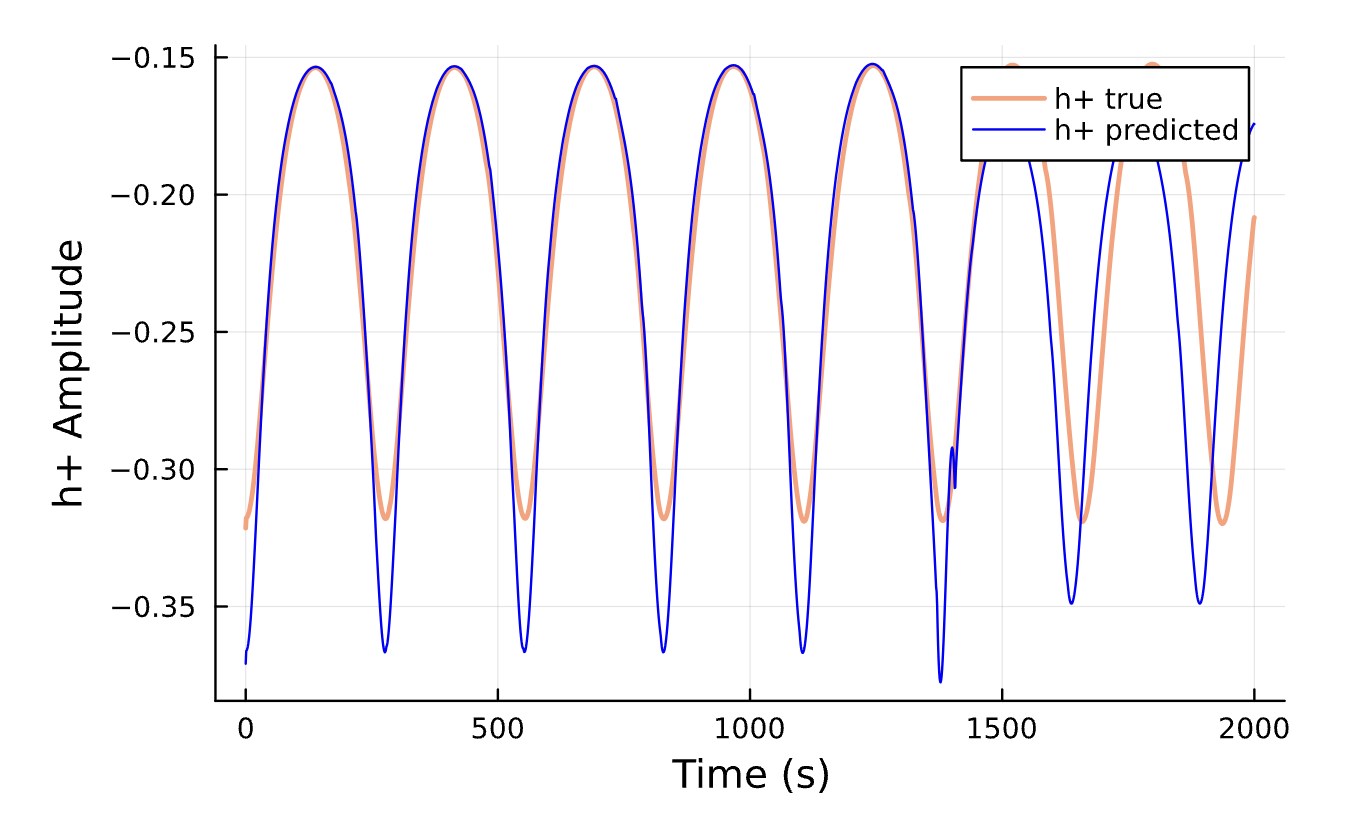
- Visualize Results
The Recipe
- Generate Training Data
- Define Hamiltonian in GENERIC Form
- Define Neural ODE
- Create Loss + Callback Functions
- Optimize over Learnable Parameters
- Iteratively Train the Optimizer
- Visualize Results
The Recipe
- Generate Training Data
- Define Hamiltonian in GENERIC Form
- Define Neural ODE
- Create Loss + Callback Functions
- Optimize over Learnable Parameters
- Iteratively Train the Optimizer
- Visualize Results
The Recipe
- Generate Training Data
- Define Hamiltonian in GENERIC Form
- Define Neural ODE
- Create Loss + Callback Functions
- Optimize over Learnable Parameters
- Iteratively Train the Optimizer
- Visualize Results
The Recipe
- Generate Training Data
- Define Hamiltonian in GENERIC Form
- Define Neural ODE
- Create Loss + Callback Functions
- Optimize over Learnable Parameters
- Iteratively Train the Optimizer
- Visualize Results
The Recipe
- Generate Training Data
- Define Hamiltonian in GENERIC Form
- Define Neural ODE
- Create Loss + Callback Functions
- Optimize over Learnable Parameters
- Iteratively Train the Optimizer
- Visualize Results
The Recipe
- Generate Training Data
- Define Hamiltonian in GENERIC Form
- Define Neural ODE
- Create Loss + Callback Functions
- Optimize over Learnable Parameters
- Iteratively Train the Optimizer
- Visualize Results
The Recipe
- Generate Training Data
- Define Hamiltonian in GENERIC Form
- Define Neural ODE
- Create Loss + Callback Functions
- Optimize over Learnable Parameters
- Iteratively Train the Optimizer
- Visualize Results
The Recipe
- Generate Training Data
- Define Hamiltonian in GENERIC Form
- Define Neural ODE
- Create Loss + Callback Functions
- Optimize over Learnable Parameters
- Iteratively Train the Optimizer
- Visualize Results
The Recipe
- Generate Training Data
- Define Hamiltonian in GENERIC Form
- Define Neural ODE
- Create Loss + Callback Functions
- Optimize over Learnable Parameters
- Iteratively Train the Optimizer
- Visualize Results
The Recipe
- Generate Training Data
- Define Hamiltonian in GENERIC Form
- Define Neural ODE
- Create Loss + Callback Functions
- Optimize over Learnable Parameters
- Iteratively Train the Optimizer
- Visualize Results
The Recipe
- Generate Training Data
- Define Hamiltonian in GENERIC Form
- Define Neural ODE
- Create Loss + Callback Functions
- Optimize over Learnable Parameters
- Iteratively Train the Optimizer
- Visualize Results
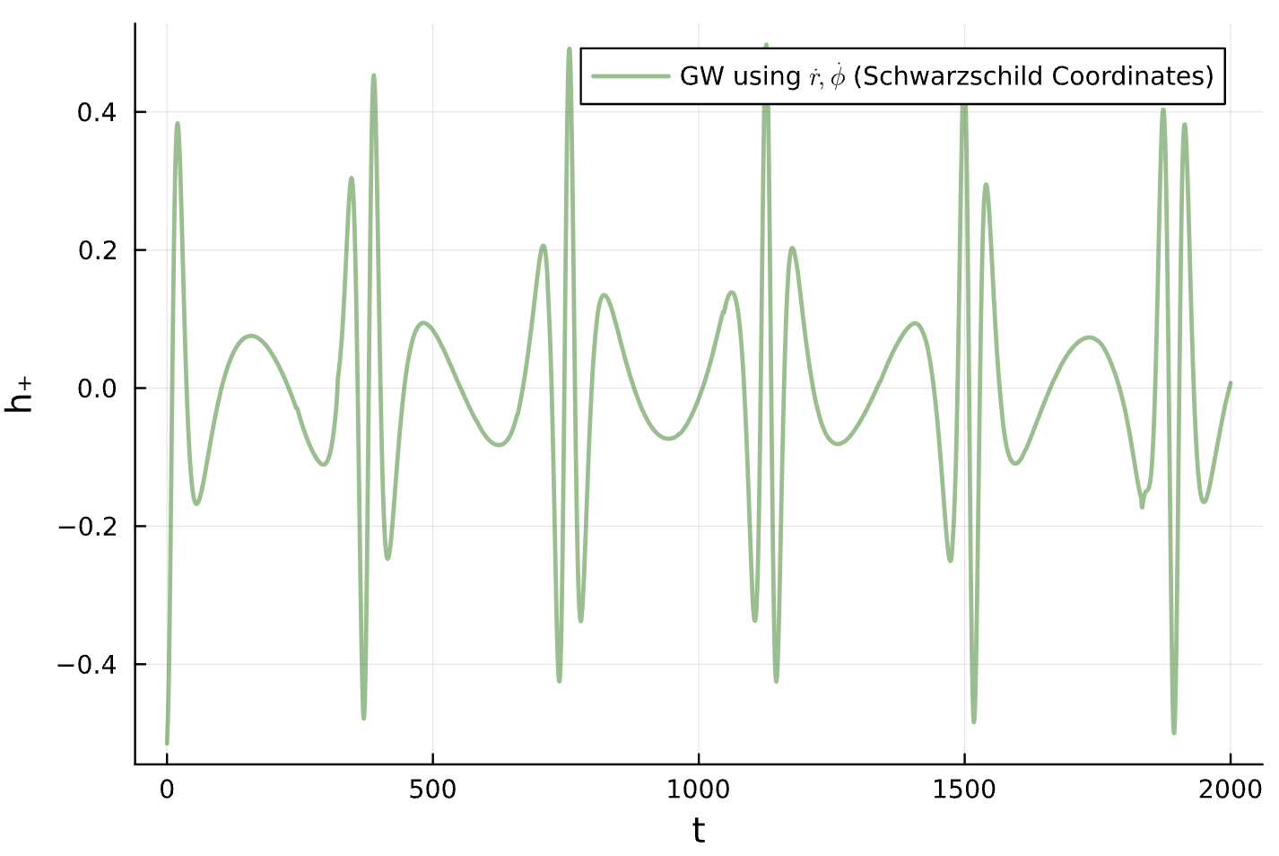
Training Data
GENERIC Hamiltonian
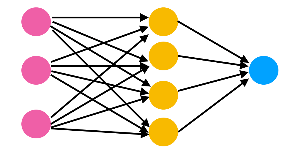
Neural ODE
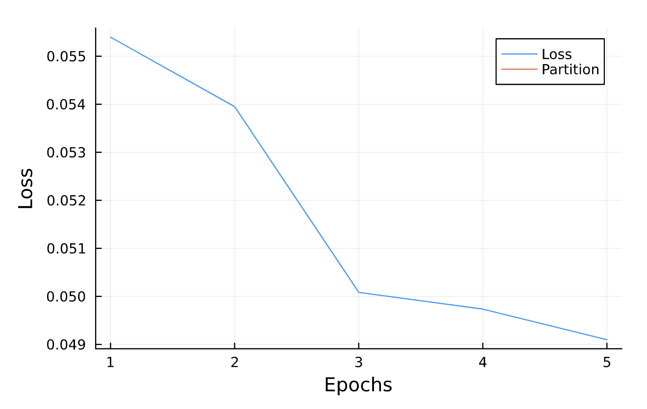
Loss + Callback
Optimizer
Training
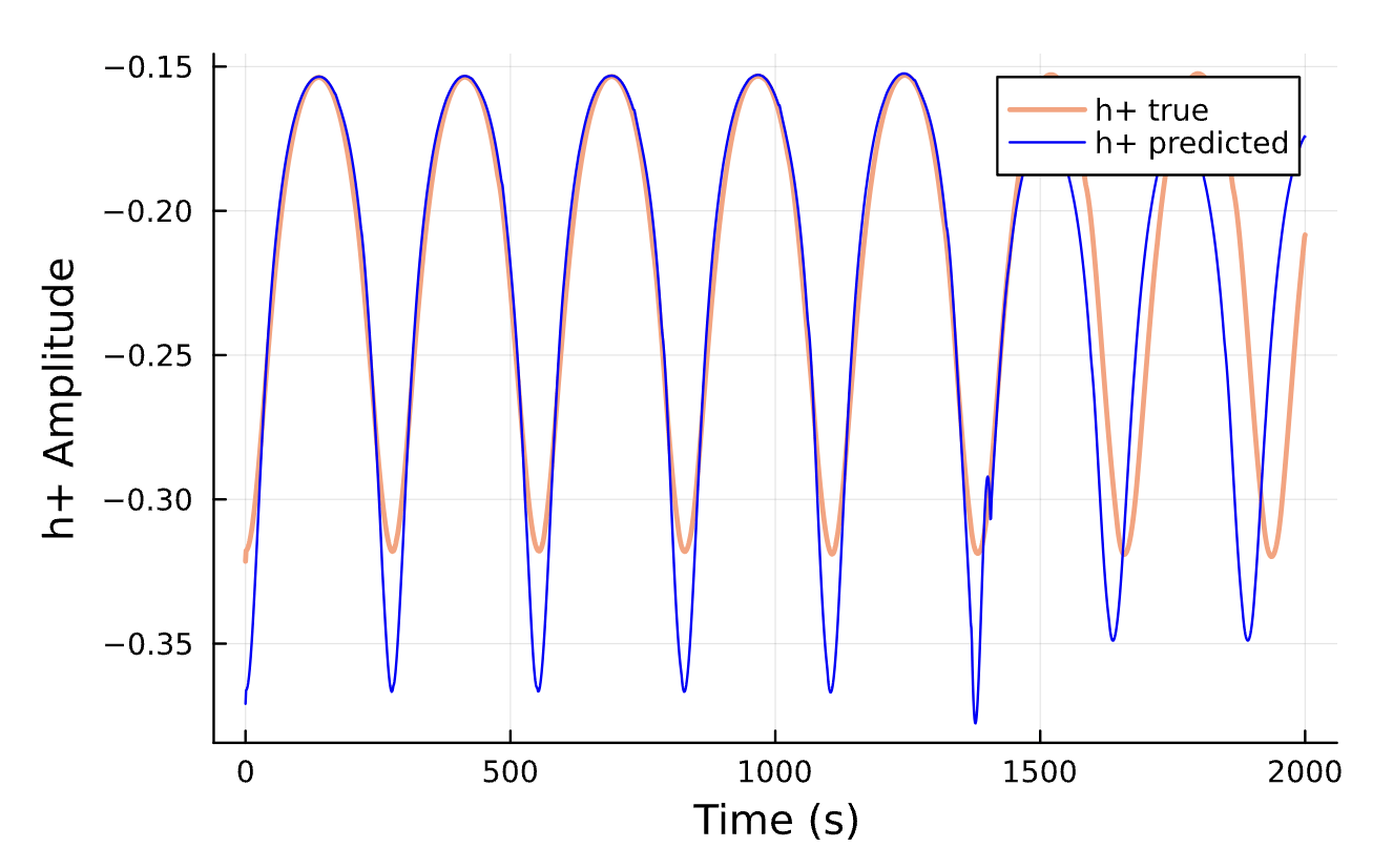
Results
Training Data
GENERIC Hamiltonian
Define Neural ODE
Loss + Callback
Optimizer
Training
Results
Training Data
GENERIC Hamiltonian
Define Neural ODE
Loss + Callback
Optimizer
Training
Results
Training Data
GENERIC Hamiltonian
Define Neural ODE
Loss + Callback
Optimizer
Training
Results
Training Data
GENERIC Hamiltonian
Define Neural ODE
Loss + Callback
Optimizer
Training
Results
Training Data
GENERIC Hamiltonian
Define Neural ODE
Loss + Callback
Optimizer
Training
Results
Training Data
GENERIC Hamiltonian
Define Neural ODE
Loss + Callback
Optimizer
Training
Results
Training Data
GENERIC Hamiltonian
Define Neural ODE
Loss + Callback
Optimizer
Training
Results
Training Data
function create_Schwarzschild_trainingData(initial_conditions)
semirectum = initial_conditions[1] # Semi-latus rectum
ecc = initial_conditions[2] # Eccentricity
function Schwarzschild_Geodesics(du, u, p, t)
coord_time, r, θ, ϕ, p_t, p_r, p_θ, p_ϕ = u # state (Schwarzschild Coordinates)
M, E, L = p # parameters (Mass, Energy, Angular Momentum)
du[1] = dt = E*(1-2*M/r)^(-1)
du[2] = dr = (1-2*M/r)*p_r
du[3] = dθ = 0
du[4] = dϕ = r^(-2)*L
du[5] = dp_t = 0
du[6] = dp_r = -(1/2)*( (1-2*M/r)^(-2)*(2*M/r^2)*(p_t)^2
+ (2*M/(r^2))*(p_r)^2
- 2*(r^(-3))*(L)^2)
du[7] = dp_θ = 0
du[8] = dp_ϕ = 0
end
M, E, L = pe_2_EL(semirectum, ecc)
R = semirectum*M/(1+ecc) # Radius of Orbit
initial_conditions()
prob = ODEProblem(Schwarzschild_Geodesics, initial_conditions())
true_sol = solve(prob, Tsit5(), saveat = timestep)
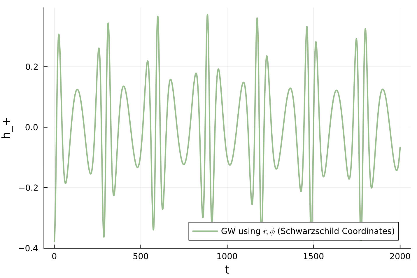
h_plus_full = compute_waveform(timestep, true_sol, 1.0; coorbital=true)[1]
h_cross_full = compute_waveform(timestep, true_sol, 1.0; coorbital=true)[2]Training Data
function create_Schwarzschild_trainingData(initial_conditions)
  semirectum = initial_conditions[1] # Semi-latus rectum
  ecc = initial_conditions[2] # Eccentricity

  function Schwarzschild_Geodesics(du, u, p, t)
      coord_time, r, θ, ϕ, p_t, p_r, p_θ, p_ϕ = u # state (Schwarzschild Coordinates)
      M, E, L = p # parameters (Mass, Energy, Angular Momentum)

      du[1] = dt = E*(1-2*M/r)^(-1)
      du[2] = dr = (1-2*M/r)*p_r
      du[3] = dθ = 0
      du[4] = dϕ = r^(-2)*L

      du[5] = dp_t = 0
      du[6] = dp_r = -(1/2)*( (1-2*M/r)^(-2)*(2*M/r^2)*(p_t)^2
                      + (2*M/(r^2))*(p_r)^2
                      - 2*(r^(-3))*(L)^2)
      du[7] = dp_θ = 0
      du[8] = dp_ϕ = 0
  end
function SchwarzschildHamiltonian_GENERIC(du, u, p, t)
        x = u
        function H(state_vec)
            t, r, θ, φ, p_t, p_r, p_θ, p_φ = state_vec
            M, E, L = p.M, p.E, p.L
            NN_params = p.NN

            H_kepler = p_r^2/2 - M/r + p_φ^2/(2*r^2)
            NN_correction = NN([r, p_r, p_φ], NN_params, NN_state)[1][1]
            return H_kepler + NN_correction
        end

        # Compute gradient using ForwardDiff
        grad_H = ForwardDiff.gradient(H, x)

        # Define symplectic matrix L (8x8)
        L = [zeros(4,4)  I(4);
             -I(4)       zeros(4,4)]

        # Hamilton's equations: ẋ = L∇H
        du .= L * grad_H

    end
GENERIC Hamiltonian
NN = Chain(Dense(3, 4, tanh), # 3 inputs: r, p_r, p_φ
            Dense(4, 4, tanh),
            Dense(4, 1)) # 1 output: Correction to H_Kepler

for layer in NN_params
  if ~isempty(layer)
    layer.weight .*= 0 .* layer.weight
    layer.bias .*= 0 .* layer.bias
  end
end


θ = (; M = p_guess[1], E = p_guess[2], L = p_guess[3], NN = NN_params)
θ = ComponentVector{precision}(θ);
prob_learn = ODEProblem(SchwarzschildHamiltonian_GENERIC, u0, tspan, θ)
Define Neural ODE
Loss + Callback
function loss(pn, trainingFraction)
newprob = remake(prob_learn, p = pn)
sol = solve(newprob, Tsit5(), saveat=timestep)
predicted_waveform_plus = compute_waveform(timestep,
sol, 1.0; coorbital=true)[1]
predicted_waveform_cross = compute_waveform(timestep,
sol, 1.0; coorbital=true)[2]
h_plus_training = trainingData[3]
h_cross_training = trainingData[4]
loss_value = sum(abs2, predicted_waveform_plus[1:n_compare]
.- h_plus_training[1:n_compare]) / n_compare +
(H - (-0.5))^2) # H should equal -1/2
return loss_value
function callback(pn, loss; dotrain = true)
if dotrain
push!(losses, loss);
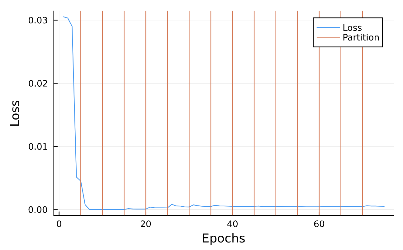
vline!(partition_boundaries, label = "Partition")function partitionTraining(numCycles, totalTrainingFraction)
global partition_boundaries, losses, final_paramaters, solutions_list, parameters_list
amountTrain = totalTrainingFraction / numCycles
p_final_array = [θ_final]
for i in 1:numCycles
trainingFraction = i * amountTrain
optf = Optimization.OptimizationFunction((x, p) -> loss(x, trainingFraction), adtype)
θ_current = p_final_array[end]
optprob = Optimization.OptimizationProblem(optf, θ_current)
opt_result_2 = Optimization.solve(optprob, Optim.BFGS(; initial_stepnorm = lr),
callback=callback, maxiters=num_iters)
θ_final_2 = opt_result_2.u;
newprob_2 = remake(prob_learn, p = θ_final_2)
sol_2 = solve(newprob_2, Tsit5(), saveat=timestep)
h_plus_pred = compute_waveform(timestep, sol_2, 1.0; coorbital=true)[1]
h_cross_pred = compute_waveform(timestep, sol_2, 1.0; coorbital=true)[2]Training
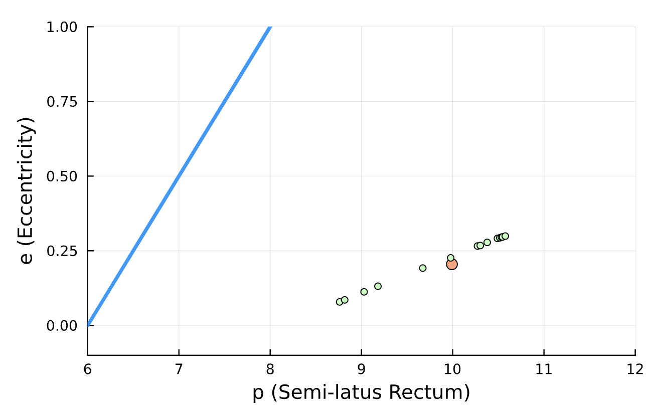
x = range(6, 12, length=20)
y = (x .- 6) ./ 2

for i in 1:numCycles
	scatter!([parameters_list[i][1]], [parameters_list[i][2]])
end

return (parameters_list[end][1] - getParameters(true_solution)[1])^2
	+ (parameters_list[end][2] - getParameters(true_solution)[2])^2

optimizeBlackHole(learningRate = 8e-3,
                  epochsPerIteration = 4,
                  numberOfCycles = 14,
                  totalTrainingPercent = 0.13,
                  true_parameters = [10, 0.2],
                  initial_guess = [10.2, 0.25])
Results
function optimizeBlackHole(; learningRate, epochsPerIteration,
							numberOfCycles, totalTrainingPercent,
							true_parameters, initial_guess)
     p_guess = pe_2_EL(initial_guess[1], initial_guess[2]) # Uses the pe_2_EL function

     trainingData = create_Schwarzschild_trainingData([true_p, true_e]) # Generate

     SchwarzschildHamiltonian_GENERIC()

     define_NN()
     initialize_weights()
     paramatersForNNToLearn()
     ODE_initialConditions()
     defineNeuralODE()

     HamiltonianConstraint()
     lossFunction()
     callback()
     optimize()

     θ_final = opt_result.u
     M_final, E_final, L_final = θ_final.M, θ_final.E, θ_final.L
     NN_params_final = θ_final.NN

     solveODEwithOptimizedParameters()
     convertSolution_2_Waveform()
     partitionTraining(numCycles, trainingFraction)
optimizeBlackHole()
create training data
define neural network
define ODE problem using NN
define loss function
optimizeBlackHole()