Spatial random graphs with tunable assortativity
Joost Jorritsma
joost.jorritsma@stats.ox.ac.uk

Intriguing maths: classical network models
Erdős–Rényi random graph \(G(n, \lambda /n)\)
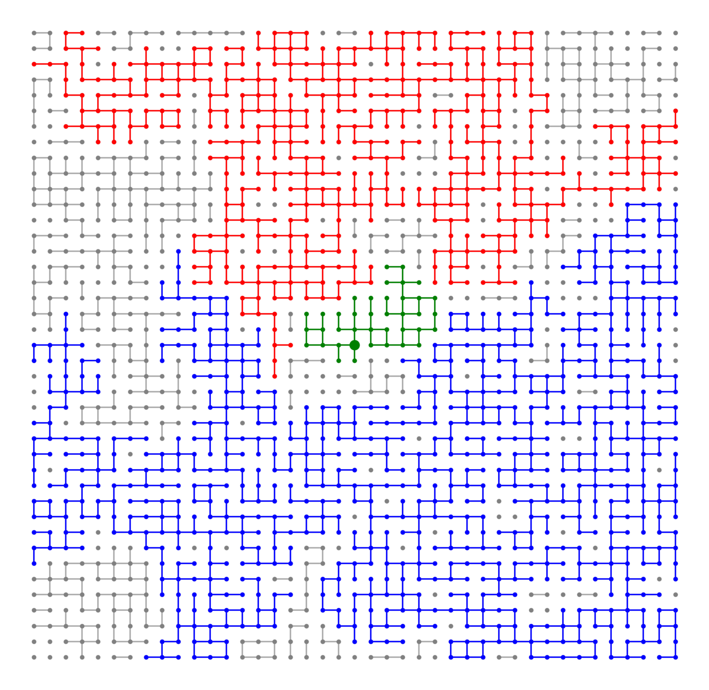
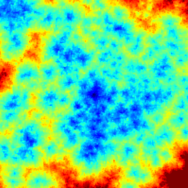
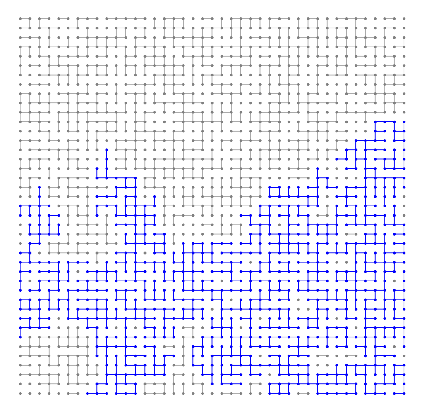
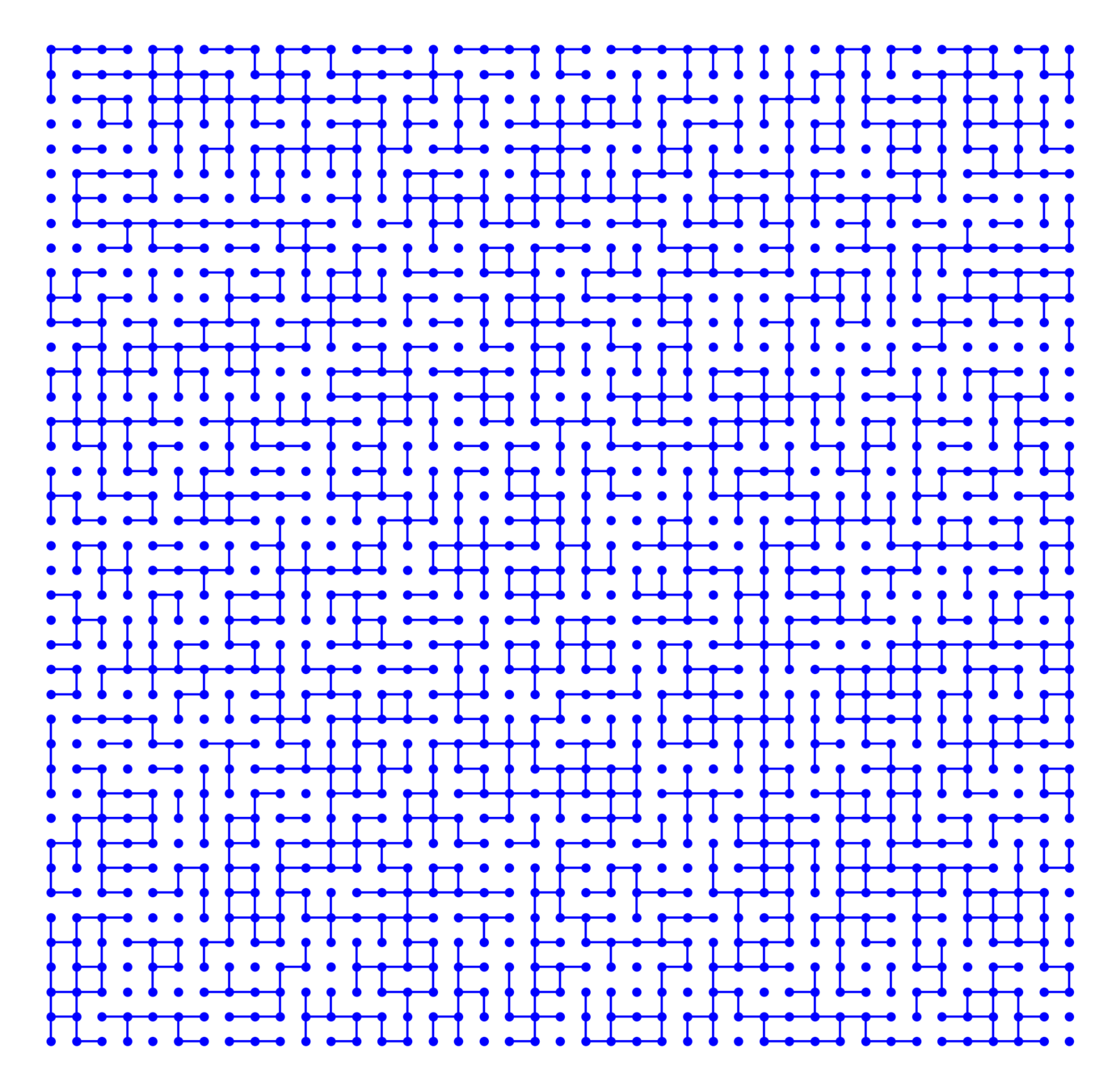
Bernoulli percolation on \(\mathbb{Z}^2\) w.p. \(p\)
Intriguing maths: classical network models
Motivation
- Do there exist graphs with property X?
- Is there a percolation phase transition?
- What happens at the critical point?
- What is the component-size distribution?
Intriguing maths: classical network models
Motivation
- Universality: do all network (models) behave like ...?
- What are the implications for real-world networks?
Aim for this talk
- Introduce model for type-1 question
- Give modelling interpretation: degree assortativity
- Is this model useful for applications?
What should we investigate?


Universal properties demand null models
- Heavy-tailed degrees (power law: \(p_k\sim k^{-\tau}\))
- Small world: small distances compared to network size
- Clustering, local communities
- Geometry: (natural) embedding of nodes into space
- Hierarchy
Adapted from Network Science (2015), A.L. Barabási
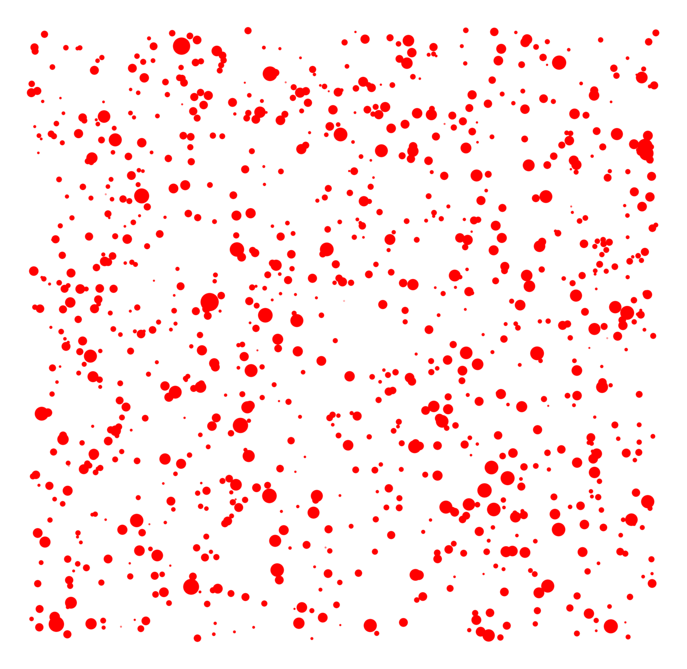
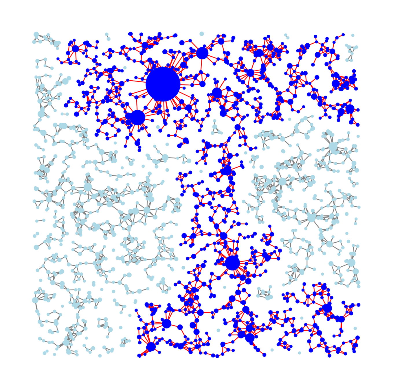
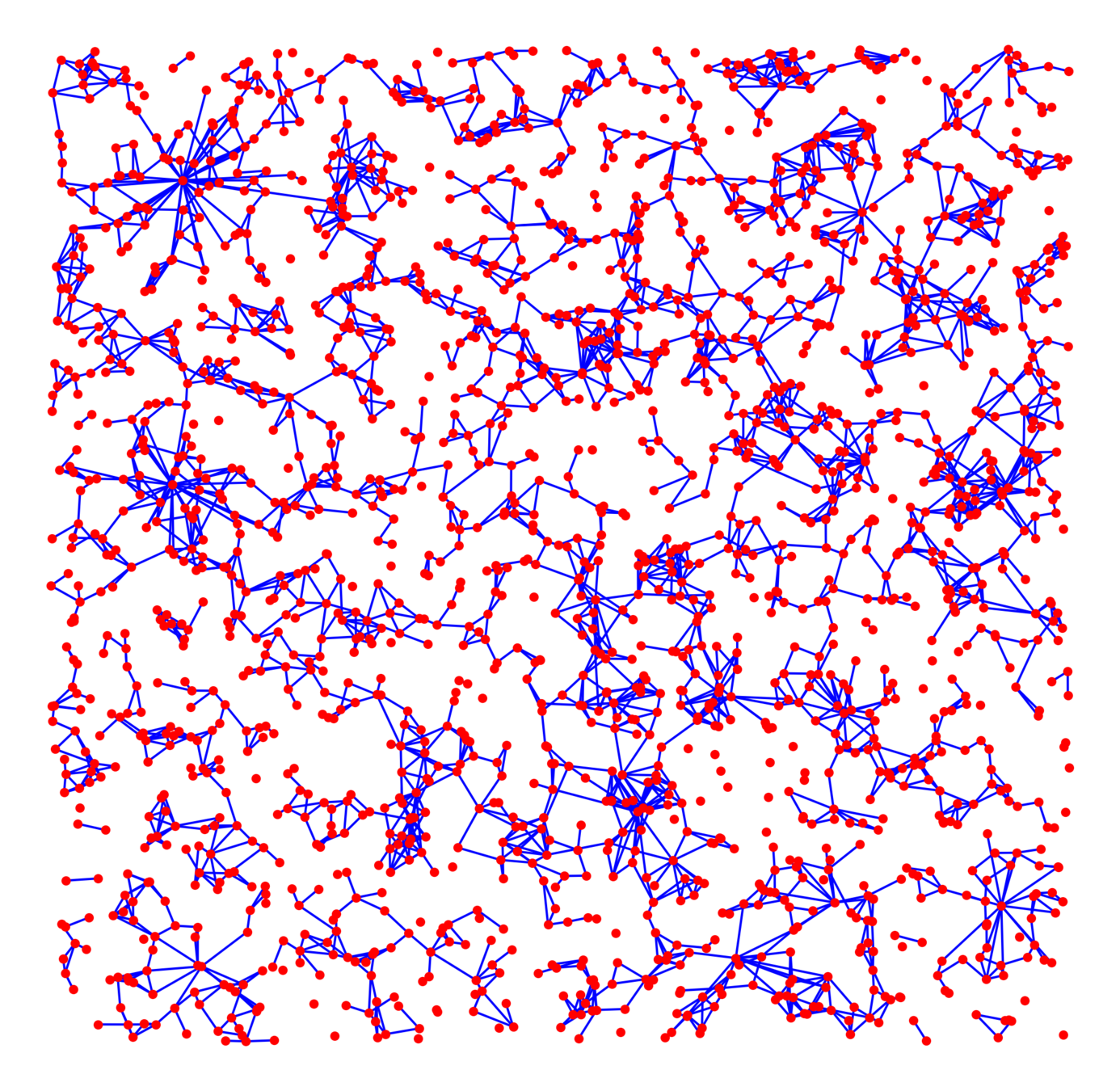
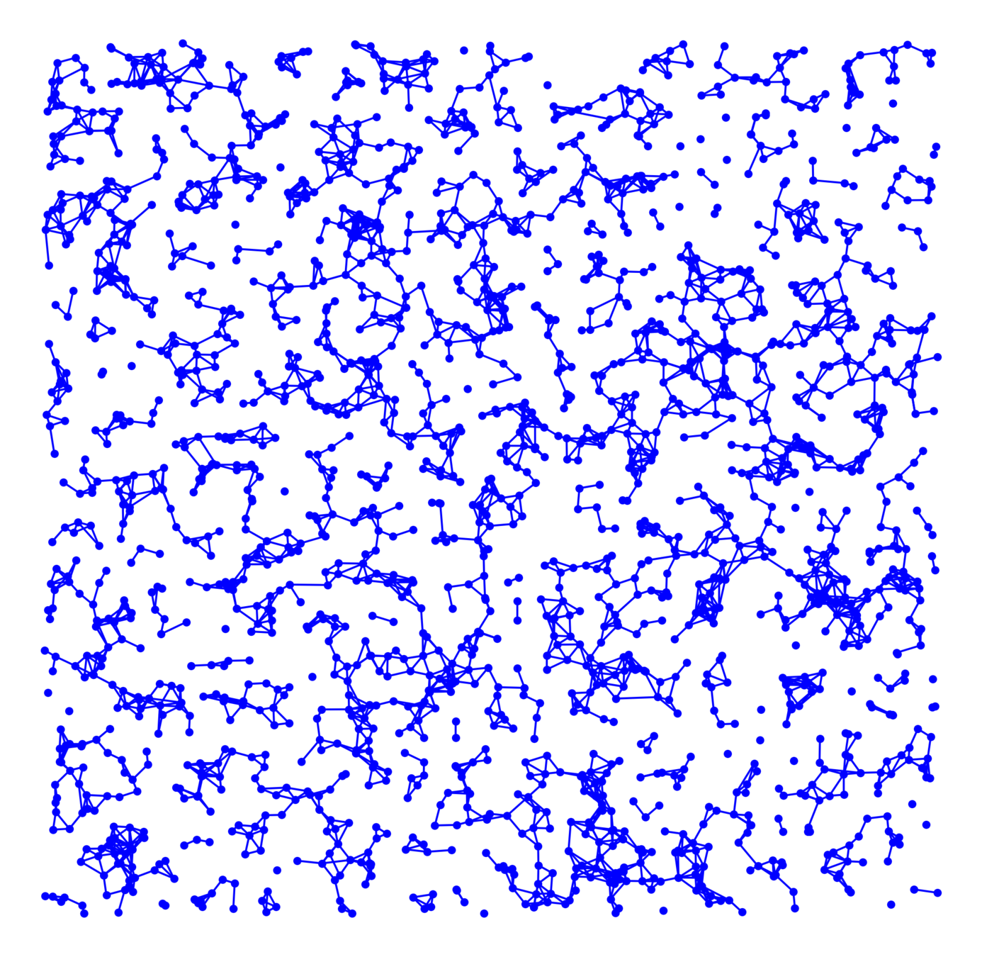
Geometric inhomogeneous random graphs (GIRG)
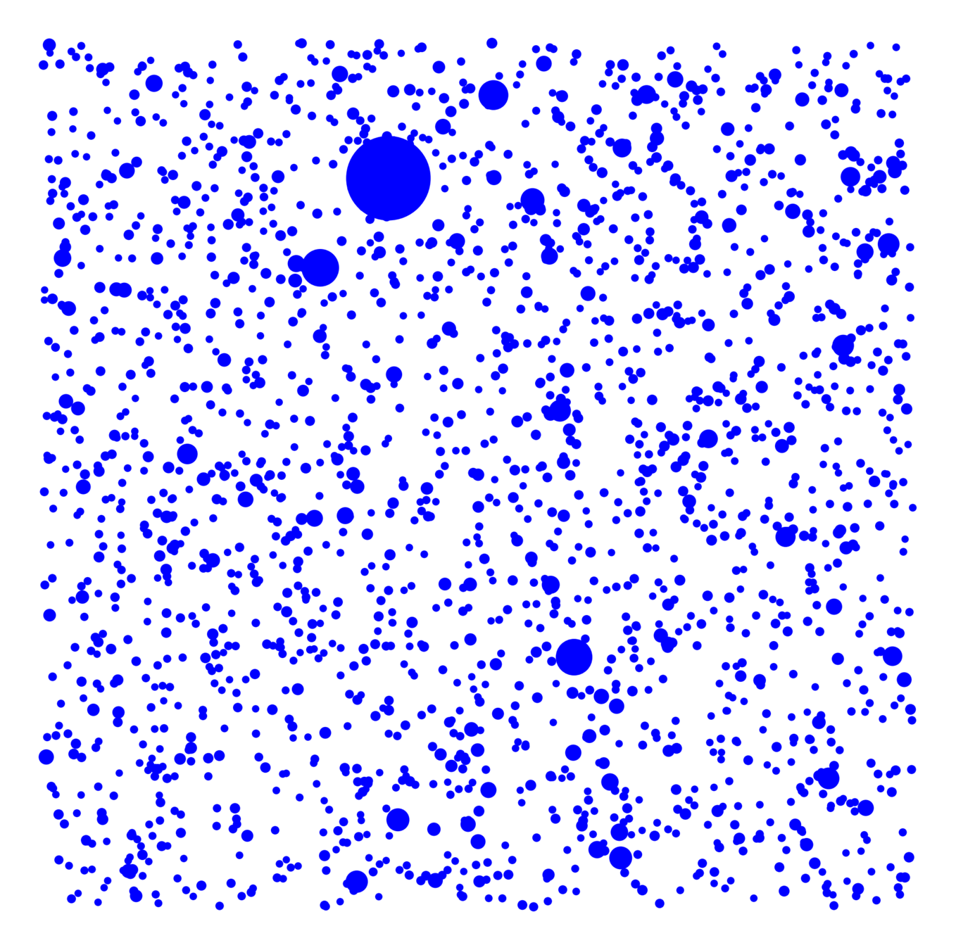
Vertex set \(\mathcal{V}_\infty\)
- Spatial locations \(x_v\in\mathbb{R}^d\)
- i.i.d. weights \(w_v\ge 1\): \(\mathbb{P}(w_v\ge w)=w^{-(\tau-1)}\),
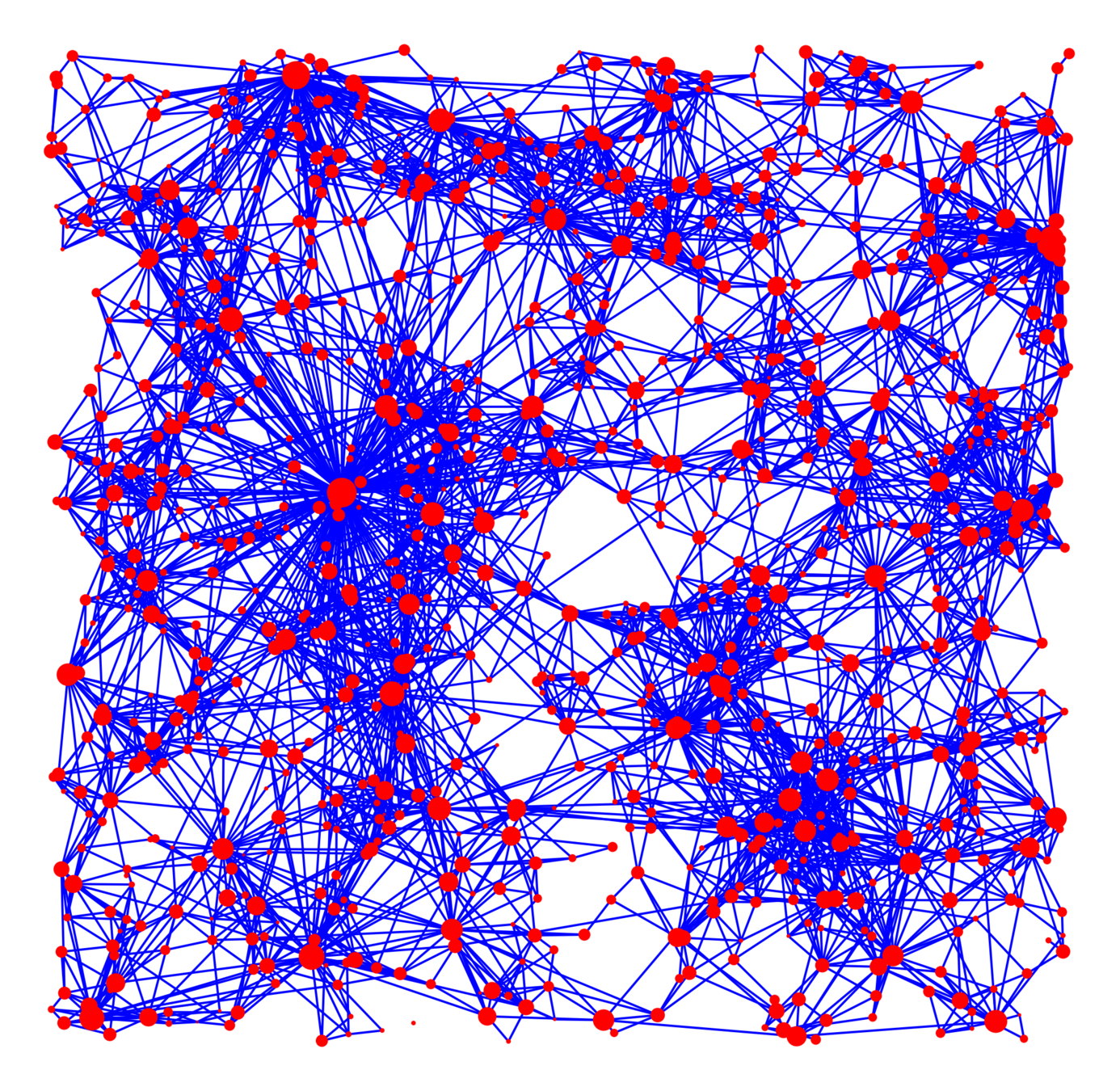
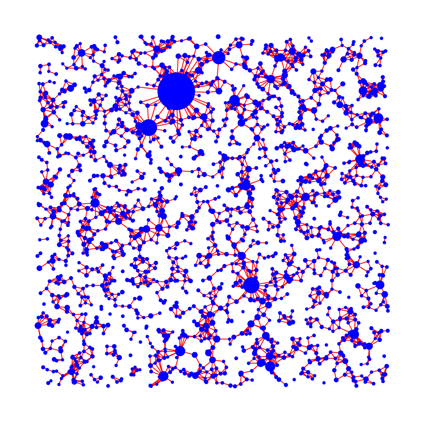
Edge set \(\mathcal{E}_\infty\)
- High weight: high degree
- Local clustering
- Long-range parameter \(\alpha>1\),
- Edge-density \(\beta>0\),
Connection probability
$$\mathbb{P}\big(u\leftrightarrow v\mid \mathcal{V}_\infty\big)=\bigg(\beta\frac{w_uw_v}{\|x_u-x_v\|^d}\bigg)^\alpha\wedge 1$$
Vertex set \(\mathcal{V}_\infty\)
- Spatial locations \(x_v\in\mathbb{R}^d\),
- i.i.d. weights \(w_v\ge 1\): \(\mathbb{P}(w_v\ge w)=w^{-(\tau-1)}\),
$$\mathbb{P}\big(u\leftrightarrow v\mid \mathcal{V}_\infty\big)=\bigg(\beta\frac{w_uw_v}{\|x_u-x_v\|^d}\bigg)^\alpha$$
$$\mathbb{P}\big(u\leftrightarrow v\mid \mathcal{V}_\infty\big)=\phantom{\bigg(\beta}\frac{w_uw_v}{\phantom{\|x_u-x_v\|^d}}\phantom{\bigg)^\alpha\wedge 1}$$
$$\mathbb{P}\big(u\leftrightarrow v\mid \mathcal{V}_\infty\big)=\phantom{\bigg(\beta}\frac{w_uw_v}{\|x_u-x_v\|^d}\phantom{\bigg)^\alpha\wedge 1}$$
$$\mathbb{P}\big(u\leftrightarrow v\mid \mathcal{V}_\infty\big)=\bigg(\phantom{\beta}\frac{w_uw_v}{\|x_u-x_v\|^d}\bigg)^\alpha\phantom{\wedge 1}$$
$$\mathbb{P}\big(u\leftrightarrow v\mid \mathcal{V}_\infty\big)$$
Geometric inhomogeneous random graphs (GIRG)
GIRG generalizes random hyperbolic graph (HRG)
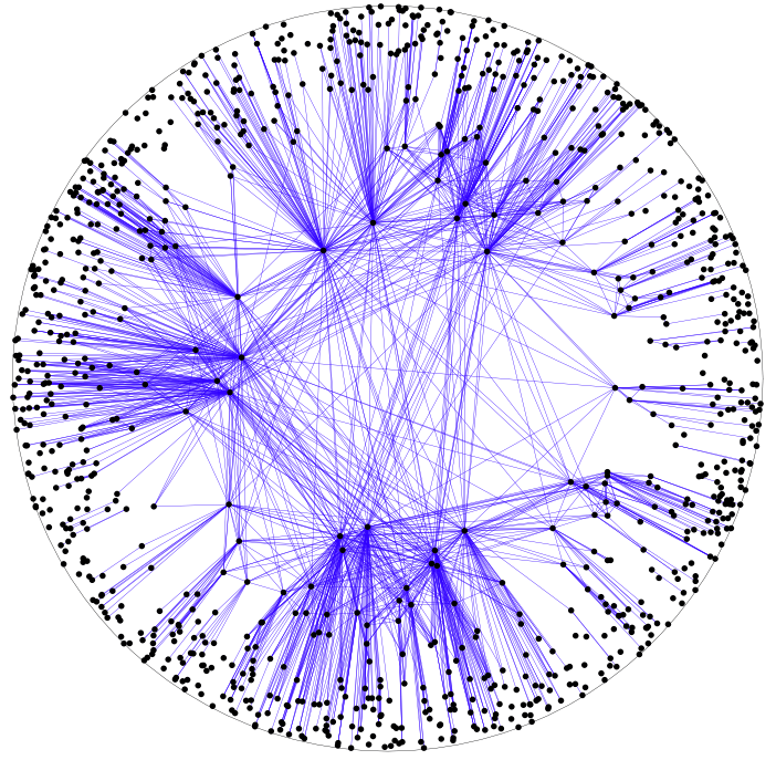
Figure by Tobias Müller
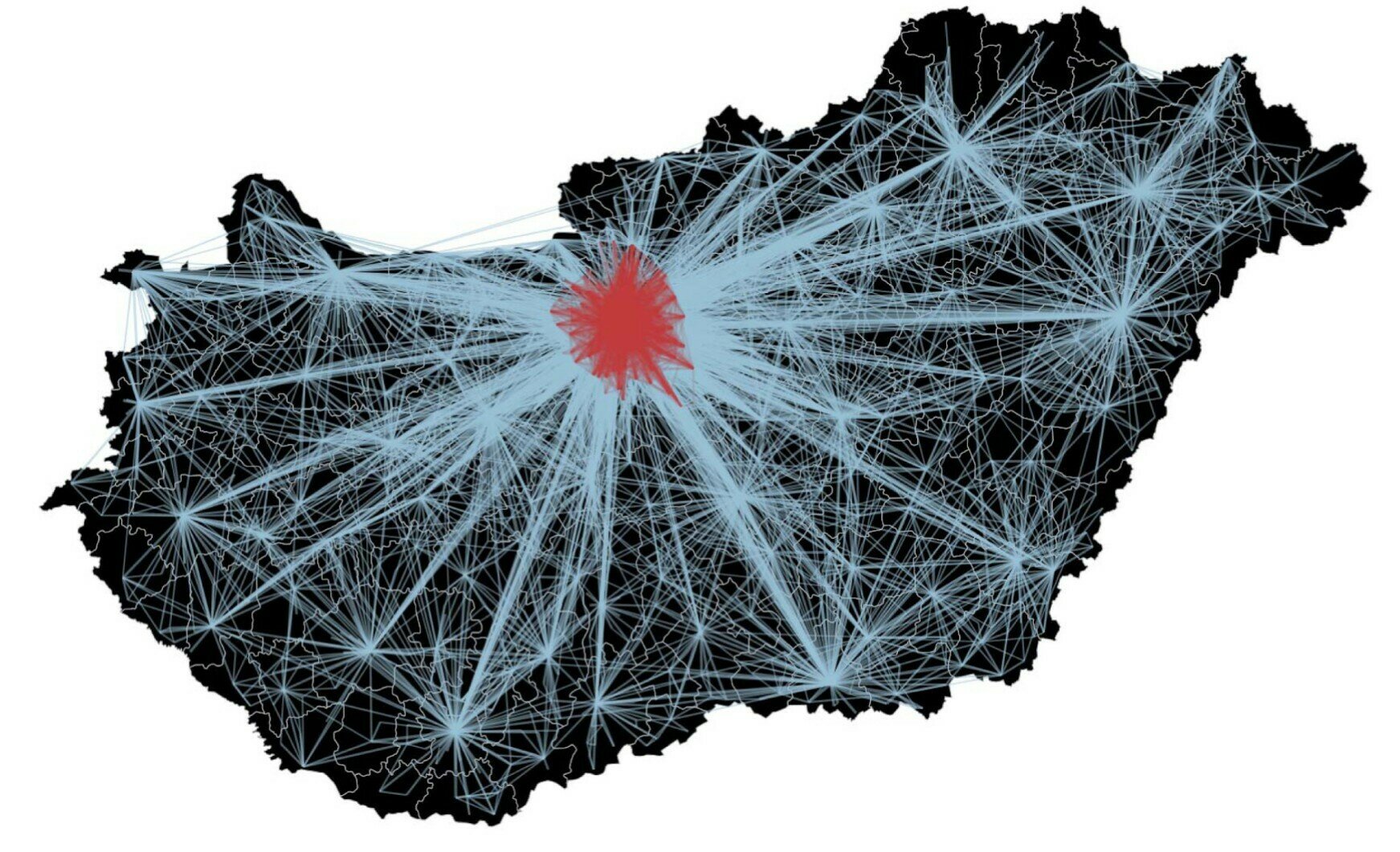
Hyperbolic random graph models Internet
Figure by Tobias Müller
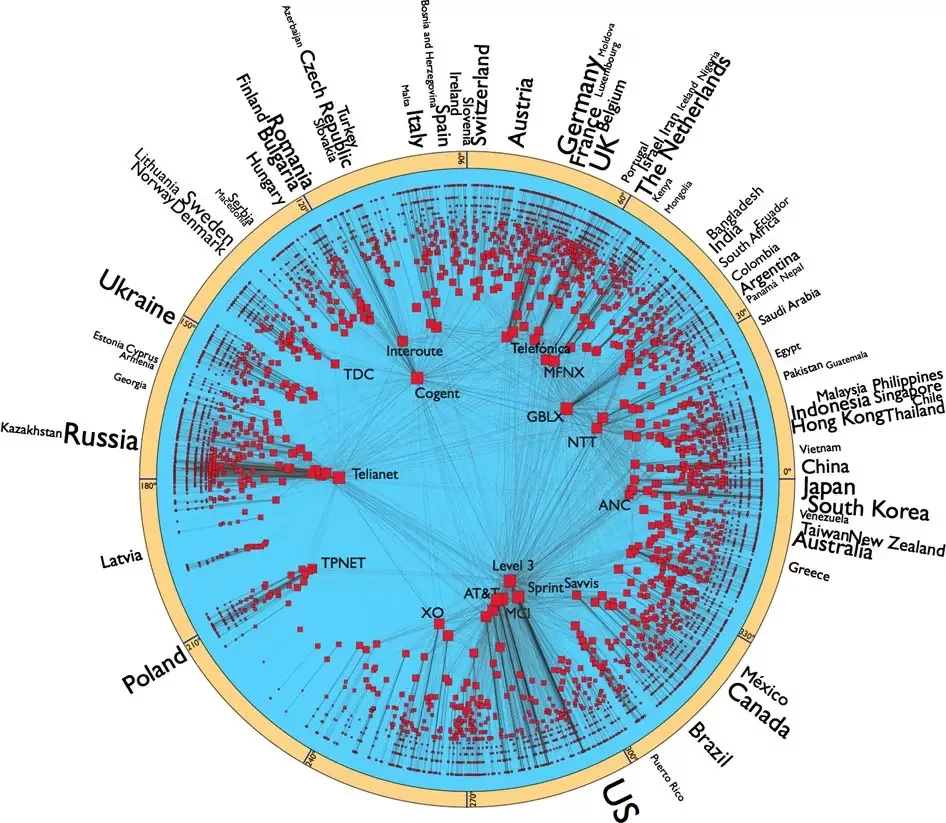
Boguñá, Papadopoulos & Krioukov (2010, Nature comm.)
GIRGs for understanding epidemics
[Odor, Czifra, Komjáthy, Lovasz, Karsai '21; Komjáthy, Lapinskas, Lengler '21]
Back to math: epidemics via percolation
Vertex set \(\mathcal{V}_\infty\)
- Spatial locations \(x_v\in\mathbb{R}^d\)
- i.i.d. weights : \(\mathbb{P}(w_v\ge w)=w^{-(\tau-1)}\),
Edge set \(\mathcal{E}_\infty\)
- Long-range parameter \(\alpha>1\),
- Edge-density \(\beta>0\),
- Percolation probability \(p\in[0,1]\)
Connection probability
$$\mathbb{P}\big(u\leftrightarrow v\mid \mathcal{V}_\infty\big)=\phantom{p\bigg(}\bigg(\beta\frac{w_uw_v}{\|x_u-x_v\|^d}\bigg)^\alpha\wedge 1\phantom{\bigg)}$$
$$\mathbb{P}\big(u\leftrightarrow v\mid \mathcal{V}_\infty\big)=p\bigg(\bigg(\beta\frac{w_uw_v}{\|x_u-x_v\|^d}\bigg)^\alpha\wedge 1\bigg)$$

Question: Is there a non-trivial phase transition?
Bernoulli percolation on \(\mathbb{Z}^2\) w.p. \(p\)
Geometric inhomogeneous random graph
Q1: Is there a non-trivial phase transition?
GIRGs contain an infinite component when
- Weights have infinite variance (\(\tau\in(2,3)\)).
- Weights have finite variance, but
enough short and long edges
(\(\alpha\in(1,2), p, \beta\) large).
- Weights have finite variance, few long edges (\(\alpha>2\)), enough short edges, and dimension at least 2.
Deijfen, vdHofstad, Hooghiemstra '13; Fountoulakis, Müller '18; Bringmann, Keusch, Lengler '19; Gracar, Lüchtrath, Mönch '25]
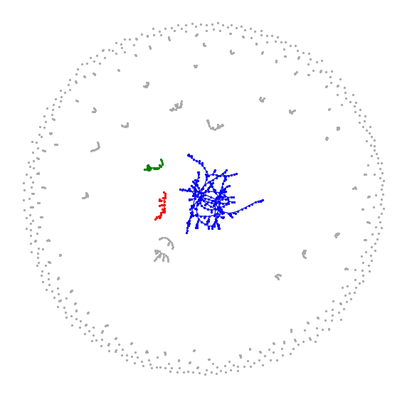
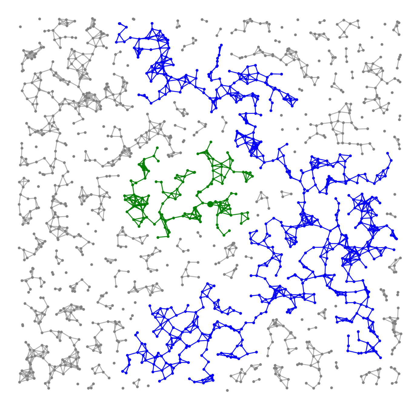
Q2: What do small components look like?
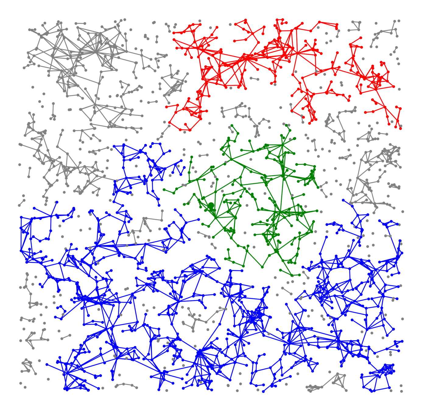
[J., Komjáthy, Mitsche '24, '24, '25]
Second-largest component,
(Finite) Component of the origin
Asymptotic size-distribution, and shape
determined by variational problem
Trade-off between
- long edges - high weights
- long edges - low weights
- short edges - dimension
\zeta=\max\bigg(\frac{3-\tau}{2-(\tau-1)/\alpha}, \,2-\alpha, \,\frac{d-1}d\bigg)
Are these the only three possible shapes?
Hyperbolic random graph
GIRG
Long-range percolation
Spatial preferential attachment
Random geom. graph
Nearest-neighbor percolation
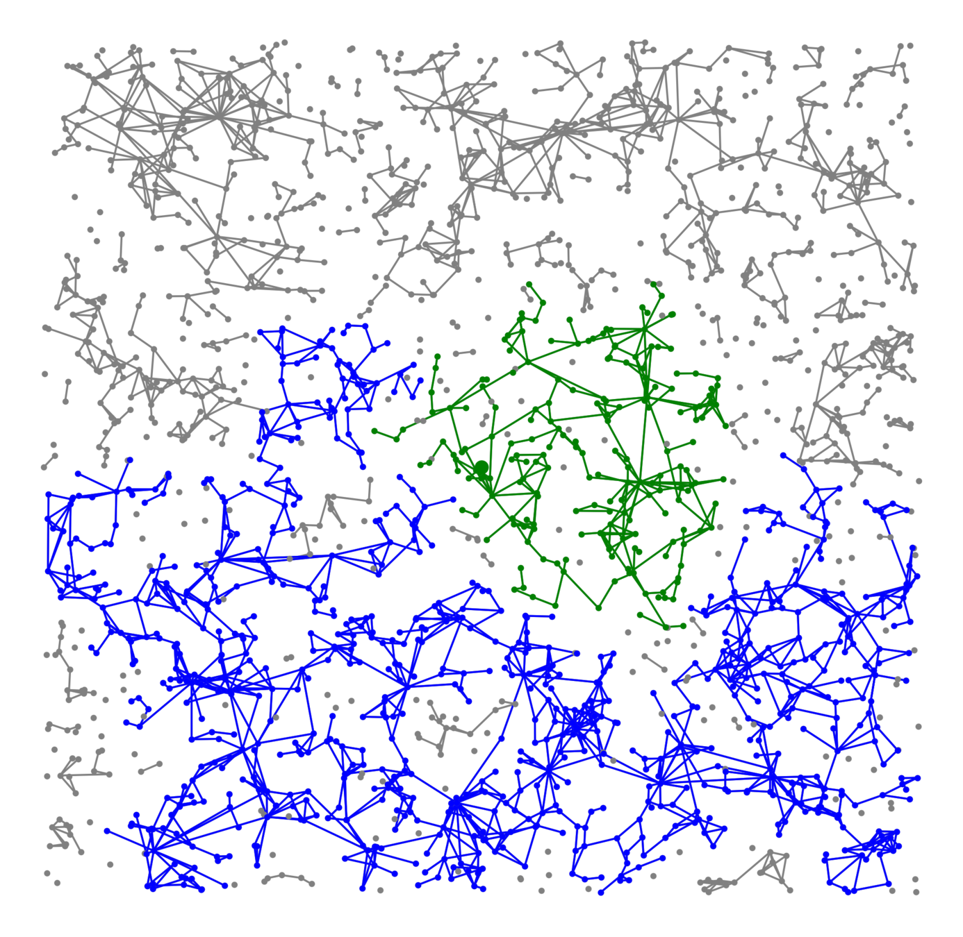
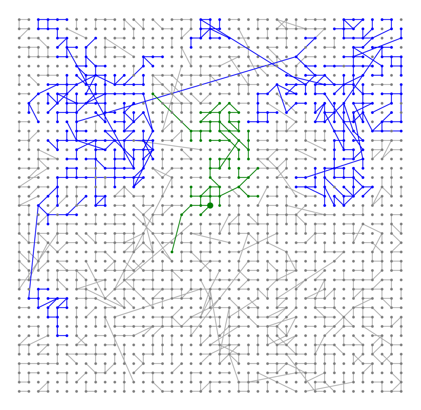
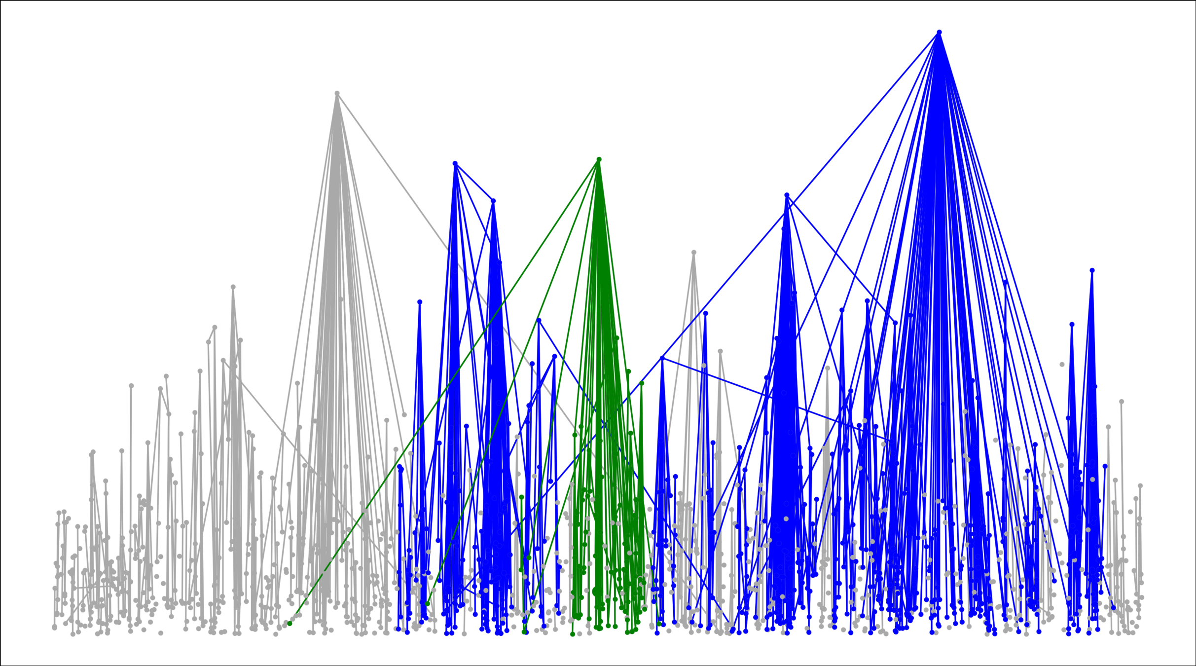
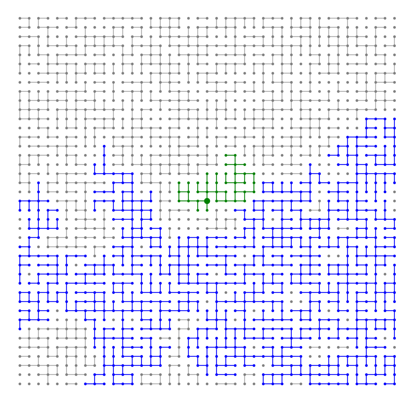
Kernel-based spatial random graphs (KSRG)
Connection probability
$$\mathbb{P}\big(u\leftrightarrow v\mid \mathcal{V}_\infty\big)=\bigg(\beta\frac{w_uw_v}{\|x_u-x_v\|^d}\bigg)^\alpha\wedge 1$$
$$\mathbb{P}\big(u\leftrightarrow v\mid \mathcal{V}_\infty\big)=\bigg(\beta\frac{\kappa(w_u,w_v)}{\|x_u-x_v\|^d}\bigg)^\alpha\wedge 1$$
Kernel \(\kappa\):
Komjáthy, Lodewijks '18; Gracar, Heydenreich, Mönch, Mörters '19; Jorritsma, Komjáthy, Mitsche '24; Gracar, Lüchtrath, Mönch '25]
The interpolating kernel generalizes many models
Connection probability
$${\color{grey}\mathbb{P}\big(u\leftrightarrow v\mid \mathcal{V}_\infty\big)=\bigg(\beta}\frac{\kappa(w_u, w_v)}{\color{grey}\|x_u-x_v\|^d}{\color{grey}\bigg)^\alpha\wedge 1}$$
A parameterized kernel: \(\sigma\ge 0\)
$$\kappa_{\sigma}(w_u, w_v):=\max\{w_u, w_v\}\min\{w_u, w_v\}^\sigma$$
- \(\tau: \mathbb{P}(w_v\ge w)=w^{-(\tau-1)}.\)
- \(\sigma\): interpolation
\frac{\sigma}{\tau-1}
\frac1{\tau-1}
1
1
\sigma=\tau-1
\tau=2
\sigma=1
\sigma=1
\sigma=\tau-2
\sigma=\tau-2
\sigma=0
\sigma=0
GIRG
Hyperbolic RG
Spatial pref. attachment
Scale-free Gilbert
Long-range percolation
Random geom. graph
Nearest-neighbor percolation
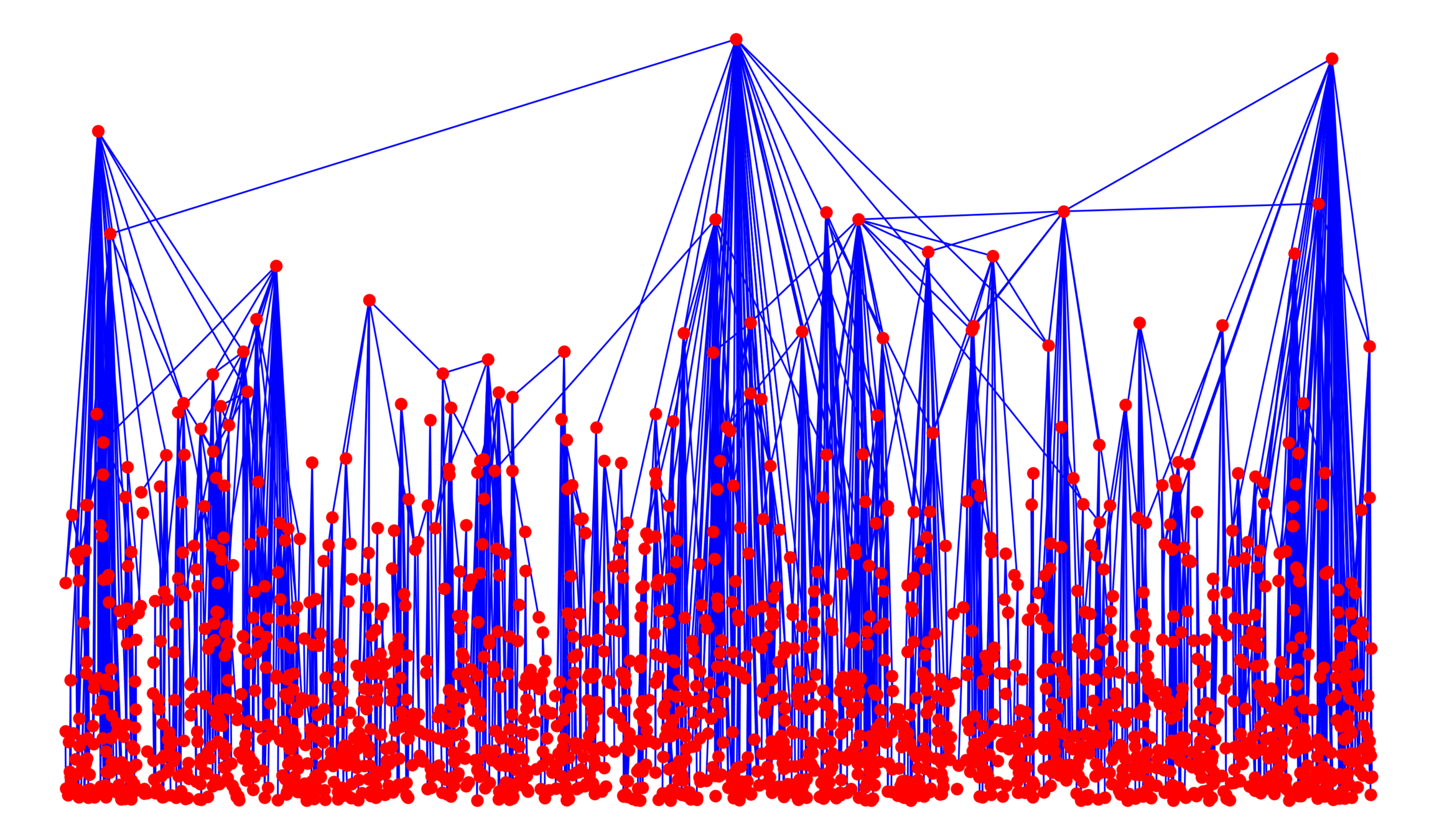
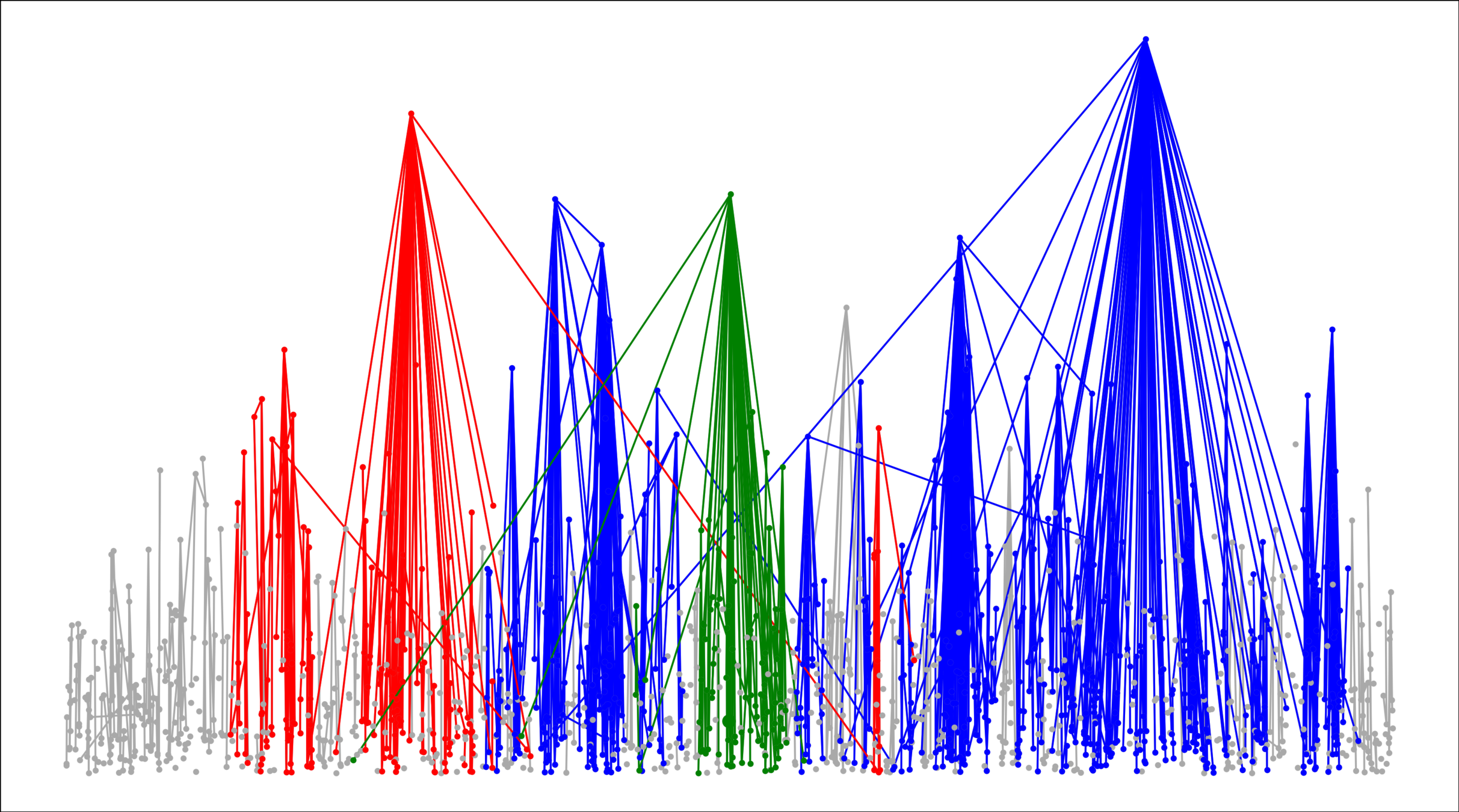
Interpolation kernel tunes degree assortativity
Connection probability
$${\color{grey}\mathbb{P}\big(u\leftrightarrow v\mid \mathcal{V}_\infty\big)=\bigg(\beta}\frac{\kappa(w_u, w_v)}{\color{grey}\|x_u-x_v\|^d}{\color{grey}\bigg)^\alpha\wedge 1}$$
A parameterized kernel, \(\sigma\in\mathbb{R}:\)
$$\kappa_{\sigma}(w_u, w_v):=\max\{w_u, w_v\}\min\{w_u, w_v\}^\sigma$$
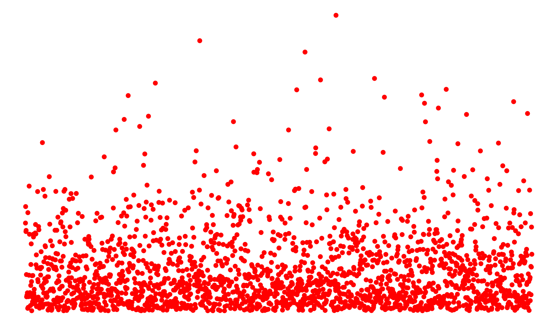
Assortativity parameter
- Weight-weight correlation of edges
- Assortativity measures similarity between endpoints of an edge
Theorem. When \(\sigma<\tau-1\) :
$$\big(\mathrm{deg}(v)\mid w_v=w\big) \sim \mathrm{Poi}(cw_v)$$
$$\mathbb{P}(w_v\ge w)=w^{-(\tau-1)},\quad \tau>2.$$
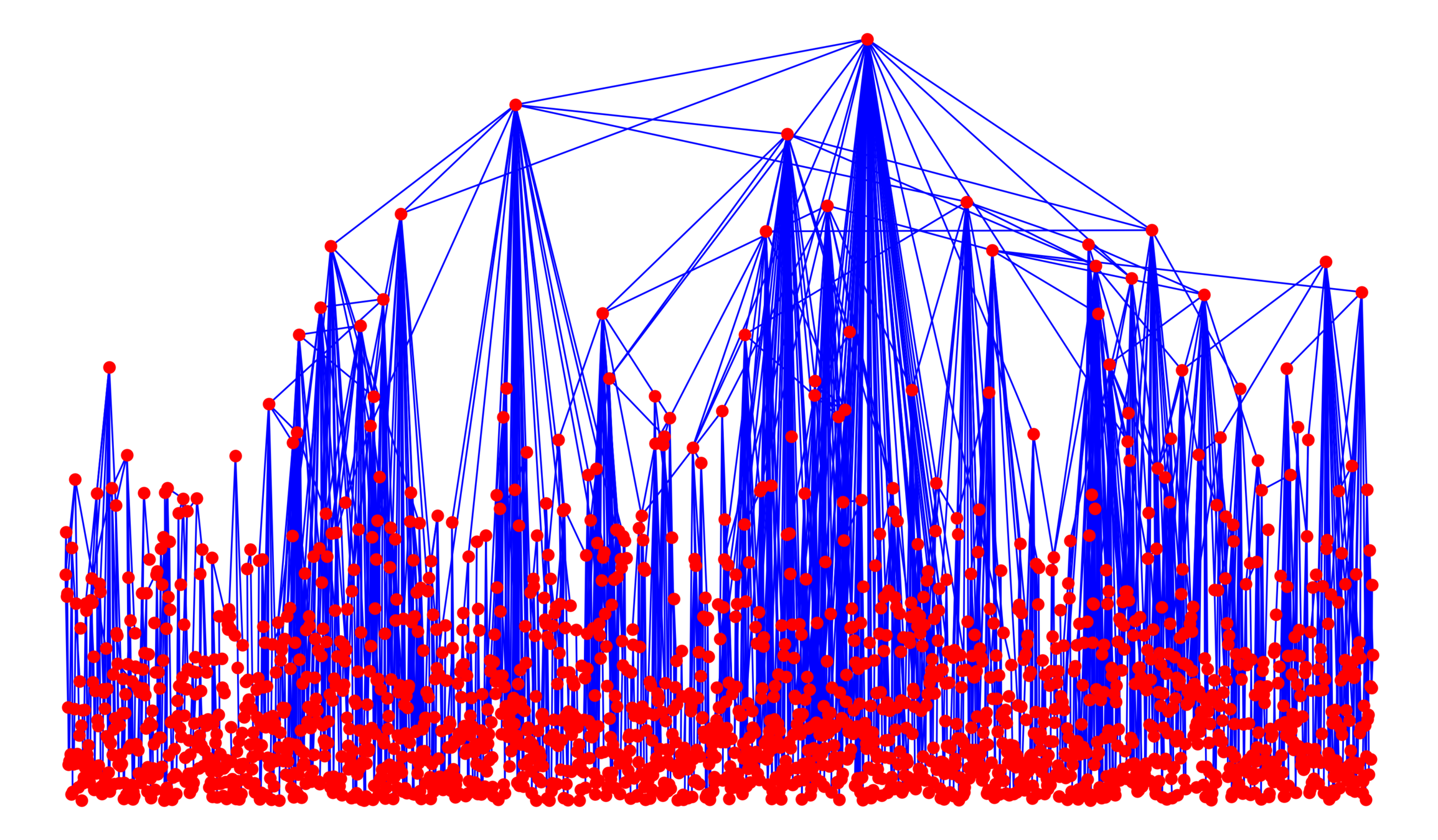
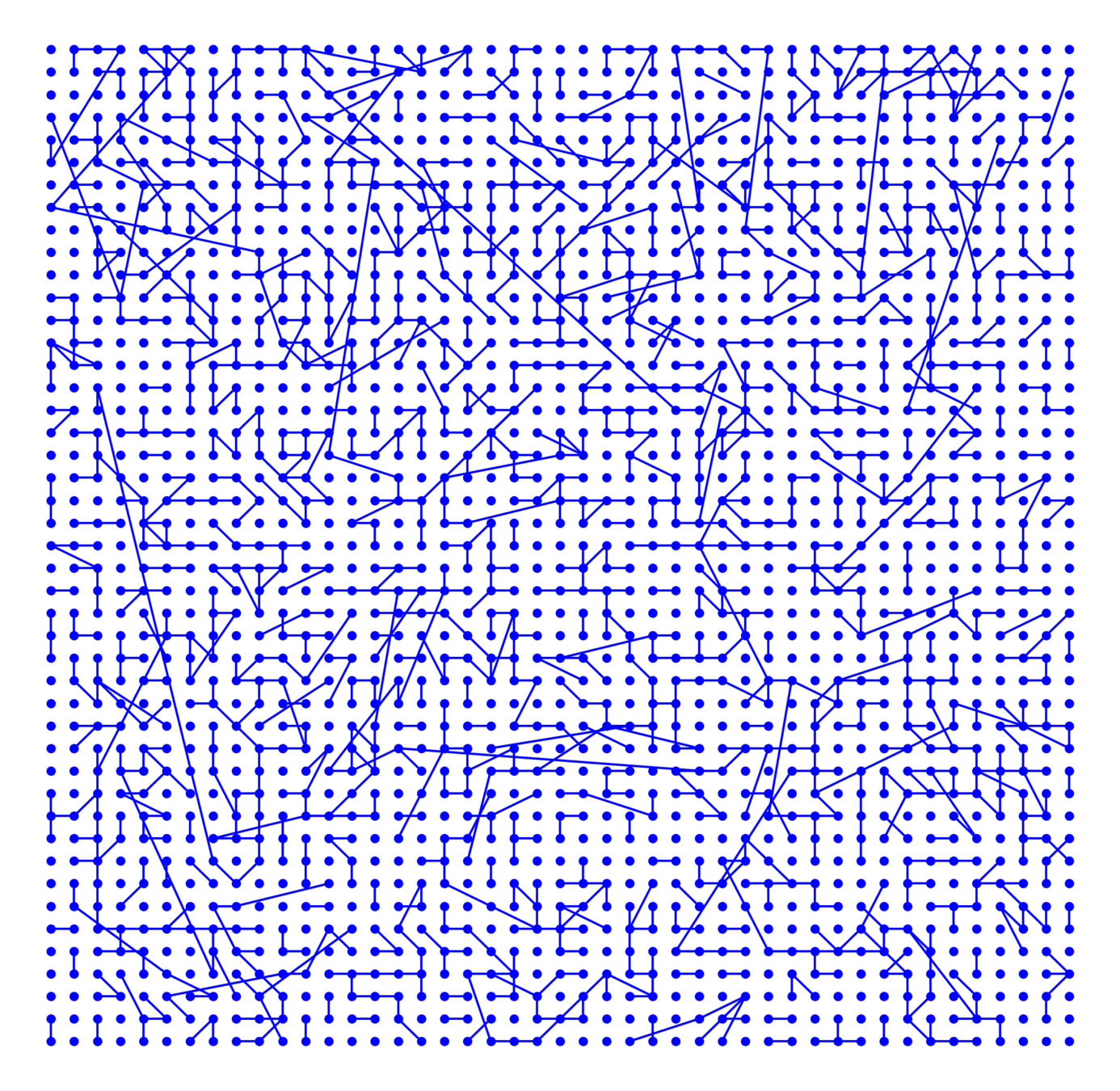
Interpolation kernel tunes degree assortativity
[Kaufmann, Schaller, Bläsius, Lengler '25+; Litvak, vdHofstad '13]
Degree-degree correlation of edges

Correlation measures
(Pearson, Spearman, Kendall)
offer less/no insight
Plots based on
$$\frac{\mathbb{P}(\mathrm{degree}(v)=y\mid \mathrm{degree}(u)=x)}{\mathbb{P}(\mathrm{degree}(v)=y)}$$
Interpolation kernel tunes degree assortativity
[Kaufmann, Schaller, Bläsius, Lengler '25+]
Degree-degree correlation of edges

Tunable GIRGs offer rich model for networks
- Heavy-tailed degrees
- Small world: small distances compared to network size
- Clustering, local communities
- Geometry: (natural) embedding of nodes into space
- Hierarchy
- Flexible degree correlations
Time for questions!
joost.jorritsma@stats.ox.ac.uk
-
Are GIRGs with tunable assortativity useful?
-
What are theoretical properties to be studied?
- Other questions?
Spatial random graphs with assortativity
By joostjor


